SPSS FOCUS
A comprehensive guide to statistical analysis in SPSS
McNemar’s Test in SPSS
McNemar’s test is a nonparametric procedure for paired or related dichotomous variables, used to determine whether the proportion of binary responses shifts across two related measurements. McNemar’s test is especially valuable in before‑and‑after study designs, where the goal is to evaluate whether an intervention, treatment, or exposure meaningfully shifted participants’ responses.
Introduction to McNemar’s Test
When comparing two related measurements, the paired samples t-test is commonly used to evaluate mean differences for paired continuous variables. In many applied research contexts—such as program evaluations and pre‑post intervention studies—data are often collected in the form of dichotomous responses rather than numeric scores. When the outcome variable reflects categories like “yes/no,” “correct/incorrect,” or “support/oppose,” the t-test becomes inappropriate. In such cases, McNemar’s test serves as the appropriate statistical method, as it evaluates whether the proportion of individuals in a given category shifts between two time points.
McNemar’s test relies on a 2×2 contingency table that cross‑classifies each participant’s responses at Time 1 and Time 2. The diagonal cells, known as concordant pairs, represent individuals whose responses remained the same across both time points and do not contribute to the calculation of the test statistic. The analysis focuses exclusively on the discordant pairs, those participants whose responses changed between measurements. McNemar’s chi‑square statistic assesses whether there is a statistically meaningful difference between the number of “yes → no” changes and the number of “no → yes” changes. A substantial disparity between these two discordant categories suggests that the intervention or condition may have influenced the distribution of responses.
McNemar’s test is appropriate whenever the same individuals provide a dichotomous response at two time points. Typical applications include public‑health interventions (e.g., willingness to get vaccinated before and after an informational session), behavior‑change programs (e.g., smoker vs. non‑smoker status before and after a cessation workshop), diagnostic comparisons (e.g., positive/negative results from two screening tools applied to the same patients), and instructional evaluations (e.g., correct/incorrect answers before and after a brief tutorial). In each case, the goal is to determine whether the proportion of people in one category has changed in a statistically meaningful way.
The data collected to perform the McNemar’s test could be in the form of raw data (Table 1) or in a summary table called a crosstab or contingency table (Table 2).
| Resident | Support (Before) | Support (After) |
|---|---|---|
| Resident 1 | Support | Support |
| Resident 2 | Support | Do Not Support |
| Resident 3 | Do Not Support | Support |
| Resident 4 | Support | Support |
| Resident 5 | Do Not Support | Do Not Support |
| … | … | … |
A crosstab or contingency table presents the sum of the counts from a raw data table.
| Opinion (Before) | Do Not Support (After) | Support (After) |
|---|---|---|
| Do Not Support | 45 | 25 |
| Support | 10 | 70 |
In the following sections, we present an example research scenario where the McNemar’s test will be used to analyze the data. We will demonstrate how to perform McNemar’s test in SPSS step-by-step and how to interpret the SPSS results for the McNemar’s test. Appendix A shows how to enter data in the form of a contingency table in SPSS.
McNemar’s Test Example
Is there a change in a condominium residents’ support for banning smoking within 25 feet of building entrances after a health‑education program?

Residents of a large condominium complex completed a survey questionnaire asking whether they support banning smoking within 25 feet of all building entrances. Before any outreach, the association distributed the initial questionnaire to capture baseline opinions. It then implemented a brief health‑education program—a set of informational materials and short presentations explaining how smoke‑free entryways reduce secondhand‑smoke exposure, improve air quality, and promote a healthier shared environment. After this program, the same residents completed the questionnaire again. Because each person provides paired, dichotomous responses (support vs. do not support), the resulting before‑and‑after data form a natural setting for McNemar’s test, which evaluates whether the health‑education program produced a meaningful shift in residents’ support for the proposed smoking‑ban rule.
| Resident | Support (Before) | Support (After) |
|---|---|---|
| Resident 1 | Support | Support |
| Resident 2 | Support | Do Not Support |
| Resident 3 | Do Not Support | Support |
| Resident 4 | Support | Support |
| Resident 5 | Do Not Support | Do Not Support |
| … | … | … |
The health researcher enters the data in the SPSS program in the computer lab. The data for this example can be downloaded in the SPSS format or in CSV format.
Entering Data into SPSS
To enter the data into the SPSS program, first we click on the Variable View tab (bottom left) and create two variables under name column: Opinion Before and Opinion After. We specify the following attributes for each variable:
- opinion_before: Type is string. Width is 24. Measure is Nominal.
- opinion_after: Type is string. Width is 24. Measure is Nominal.
When defining the variables, we must specify both the data type and the measurement level for SPSS. The data type is used by the computer to read the data, while the measurement level is used by the statistical program for computation. After creating all the variables, the Variable View panel of SPSS for our dataset should look like Figure 1 below.

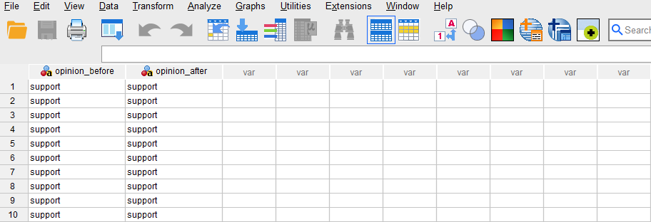
After creating the variables, we can fill in the values in the Data View tab of SPSS program. The recorded values are “Support” and “Don’t Support” before and after receiving the health education program about the risks of tobacco use. Figure 2 shows how the data for the two variables should look like in the Data View tab.
Now we are ready to run McNemar’s test in SPSS!
Analysis: McNemar’s Test in SPSS
The McNemar test is a statistical method used to evaluate changes in paired categorical responses—specifically when each participant provides a dichotomous (yes/no, correct/incorrect) answer at two time points. Instead of examining relationships between two independent categorical variables, McNemar’s test focuses on before‑and‑after data from the same individuals. In this example, we want to know if the health education program was effective by analyzing the before-after change in opinion about banning smoking using McNemar’s test.
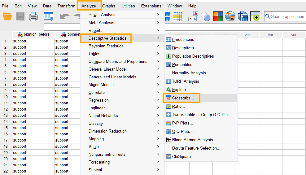
In SPSS, the McNemar’s test can be accessed through the menu Analyze / Descriptive Statistics / Crosstabs. So, as Figure 3 shows, we click on Analyze and then choose Descriptive Statistics and then Crosstabs item.
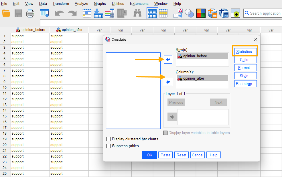
After clicking on Crosstabs, a window will appear asking for Row(s) and Columns (Figure 4). We send opinion_before to the Row(s) and opinion_after to the Column(s) boxes. Although the choice of which variables to send to the row or column will not affect the analysis results, it is good practice to send the pre-treatment variable to the rows and the post-treatment variable to the columns.
Next, in this window we click on Statistics and in the new window select McNemar (Figure 5).
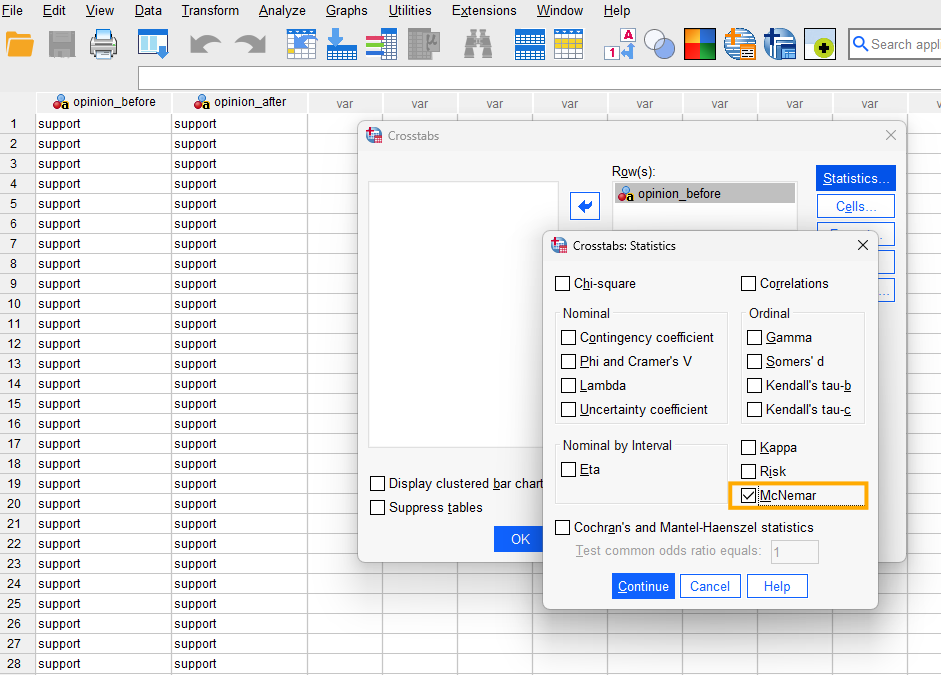
We press Continue and finally click on OK to run the McNemar’s test. SPSS will produce the results in the Output window.
Interpreting McNemar’sTest in SPSS
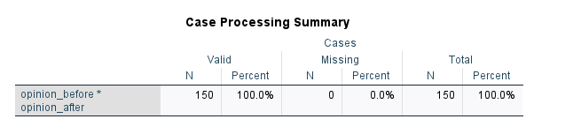
In our example, we are interested in understanding if the residents of a condominium complex change their opinion about banning smoking within 25 feet of the buildings. We collected binary response (support / don’t support) before and after running a health education program. Because the data are binary and we are interested in knowing if the residents changed their opinion, we run a McNemar’s test. The first table (Figure 6 below) from SPSS output shows the number of cases (respondents) in the data set (valid, missing, and total).
The second table (Figure 7 below) shows the crosstab or the contingency table.
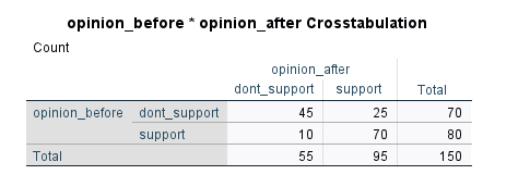
In this example, the 2×2 crosstab displays how each respondent’s opinion changed from before to after the intervention. The diagonal cells show the participants whose opinions stayed the same: 45 people did not support the policy at either time point, and 70 consistently supported it. The off‑diagonal cells contain the discordant pairs, which are the only counts used in McNemar’s test. Here, 25 individuals shifted from not supporting the policy before to supporting it after, while 10 moved in the opposite direction—from support to not support. These two discordant counts (25 vs. 10) form the basis of the McNemar chi‑square statistic and indicate whether the change in support is statistically significant.
The results of the McNemar’s test are displayed in the last table (Figure 8).
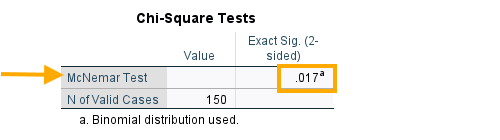
The McNemar’s test is significant (p = 0.017) supporting the effectiveness of the health education program in changing the residents’ opinion to support the banning of tobacco use within 25 feet of the buildings in the condominium complex. Note: SPSS used the binomial distribution instead of the chi-squared distribution. Binomial distribution-based test is exact while chi-squared distribution test is approximation (large samples).
Reporting McNemar’s Test Results
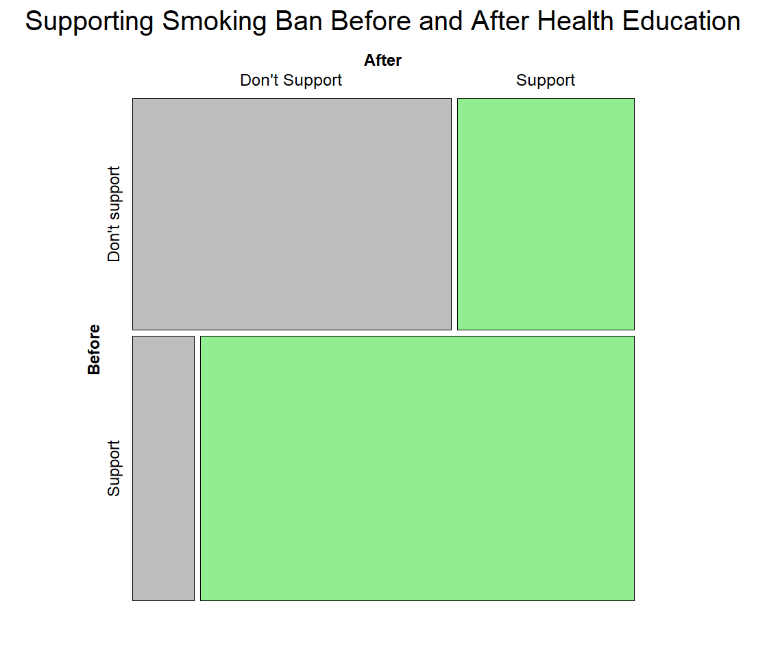
A McNemar test was conducted to examine whether support for the policy changed from before to after the intervention. Results showed a significant difference in the proportion of participants who changed their opinion (p = .017). Specifically, more individuals shifted from not supporting the policy to supporting it (25 participants) than shifted from support to not support (10 participants). These results indicate that the intervention was associated with a meaningful increase in policy support.