SPSS FOCUS
A comprehensive guide to statistical analysis in SPSS
Two-way Mixed Repeated Measures ANOVA in SPSS
A two‑way mixed repeated measures ANOVA is a statistical method used to examine if the mean measurements across two or more than two occasions or conditions are significantly different from each other and significantly different between two or more than two groups measured on those times or occasions (e.g., male vs. female). In other words, participants who are measured on multiple times belong to different groups. In this design, one factor is measured repeatedly within the same individuals (the within‑subjects factor), while the second factor (group) represents different groups (the between‑subjects factor). The two-way mixed repeated measures ANOVA design extends paired‑samples t‑test and one‑way repeated measures ANOVA by allowing researchers to test not only overall change over time but also whether different groups follow different trajectories.
Introduction to Two-way Mixed Repeated Measures ANOVA
Repeated measures designs are commonly used when researchers collect data from the same experimental units (e.g., patients, students, mice) at several time points or under several conditions (e.g., different amounts of medications or light sources). Because in this design measurement are derived from the same experimental unit, there is dependency in data and the standard methods that assume independence are not appropriate. Repeated measures ANOVA provides a framework for analyzing these dependent observations through a covariance structure while assessing how a continuous outcome changes over time or across conditions.
In addition, if the experimental units belong to different groups (e.g., outpatients and inpatients, fifth grade and sixth grade students, lean mice and fat mice), we can enter a second independent variable as a grouping factor to measure if there is a significant difference between the groups at each time point or on average. A two‑way mixed repeated measures ANOVA extends the one‑way repeated measures model by incorporating both a within‑subjects factor (e.g., time or occasions) and a between‑subjects factor (e.g., grade or sex). This allows the researcher to test overall change, group differences, and—most importantly—whether the pattern of change differs between groups. This design is called mixed because it involves change both within participants and between participants.
Two-way mixed repeated measures ANOVA is extensively used in animal studies, clinical research, public health, and psychology. By modeling both within‑person change and between‑group differences simultaneously, the two‑way mixed repeated measures ANOVA provides a comprehensive view of how an outcome evolves and whether those changes depend on group membership.
In the following sections, we present an example research scenario where a two-way mixed repeated measures ANOVA will be used to analyze the data. We will demonstrate how to perform a two-way mixed repeated measures ANOVA in SPSS step-by-step and how to interpret the SPSS output results.
Two-way Mixed Repeated Measures ANOVA Example
Does a mindfulness program help lower stress among hospital staff, and does it have equal effect on nurses and physicians?

Upon monitoring stress levels among hospital staff, the HR department decides to pilot a stress management program using mindfulness. The HR department is also interested in understanding if the mindfulness program is equally effective for both nurses and physicians.
Following the research approval from the IRB, the HR recruits 25 nurses and 25 physicians into the program. The mindfulness program lasted six months. Stress level was measured at baseline (program entry), after three months, and once again at sixth month (exit) using a psychometrical valid and reliable measure. Because each participant was measured at three time points, and because each participant belonged to two distinct groups (nurses and physicians), the study followed a two‑way mixed repeated measures design with one within‑subjects factor (Time) and one between‑subjects factor (group). Table 1 below shows the stress scores for five participants measured at three time points.
| ID | Role | Stress Time 1 | Stress Time 2 | Stress Time 3 |
|---|---|---|---|---|
| 1 | Nurse | 16 | 12 | 12 |
| 2 | Nurse | 24 | 10 | 12 |
| 3 | Nurse | 18 | 16 | 9 |
| 35 | Physician | 13 | 10 | 8 |
| 36 | Physician | 28 | 18 | 16 |
| … | … | … | … | … |
The researcher aims to evaluate whether participation in the hospital mindfulness program leads to meaningful reductions in staff stress levels and to assess if the change in stress levels is different between nurses and physicians. Stress level was measured at three intervals, and the resulting scores were entered into SPSS for analysis using a two‑way mixed repeated measures ANOVA. The dataset used in this example is available for download in both SPSS or CSV formats.
Entering Data into SPSS
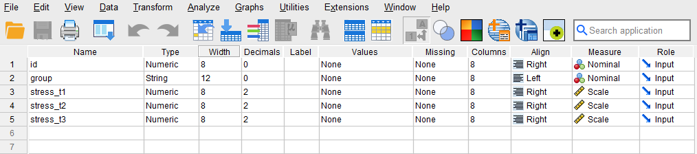
To enter the data in the SPSS program for this example, we begin by clicking on the Variable View tab (located at the bottom left of SPSS window) and create the following variables under the “Name” column: ID, group, stress_t1, stress_t2, and stress_t3. Next, we assign the following attributes to each variable:
- ID: Type is Numeric. Width is 8. Measure is Nominal.
- group: Type is String. Width is 12. Measure is Nominal.
- stress_t1: Type is Numeric. Measure is Scale.
- stress_t2: Type is Numeric. Measure is Scale.
- stress_t3: Type is Numeric. Measure is Scale
When creating variables in SPSS, it is essential to define both the data type and the measurement level. The data type determines how the software processes the input data, while the measurement level guides the statistical algorithms used for analysis.
After creating all variables, the Variable View panel of SPSS for our dataset should look like Figure 1.
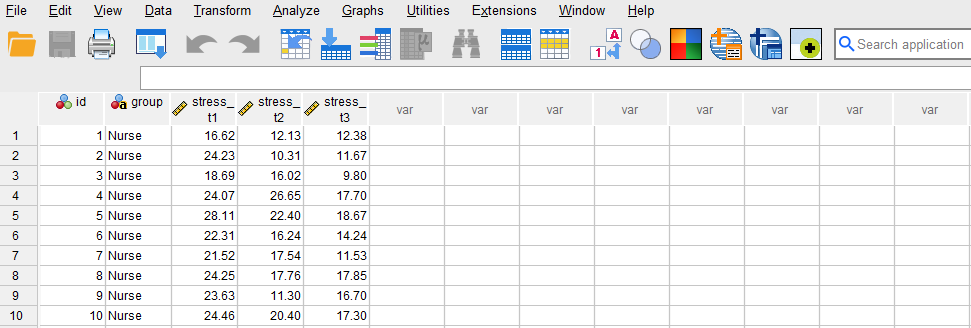
Once the variables are created, we switch to the Data View tab of the SPSS program and enter the data into the columns ID, group, stress_t1, stress_t1, and stress_t1. Figure 2 shows how the data for all four variables should look like in the Data View tab.
Now we are ready to conduct the two-way mixed repeated measures ANOVA in SPSS!
Analysis: Two-way Mixed Repeated Measures ANOVA in SPSS
A two‑way mixed repeated measures ANOVA is used when researchers want to examine how an outcome changes across multiple time points and whether those changes differ between groups of participants. In this study, the researcher is interested in understanding whether a hospital‑based mindfulness program reduces staff’s stress over time and whether this pattern of change varies between nurses and physicians. Stress levels are measured at three intervals—Time 1 (program initiation), Time 2 (three months), and Time 3 (six months). Because each participant provides repeated measurements over time and belongs to one of two roles, a mixed repeated measures design is appropriate.
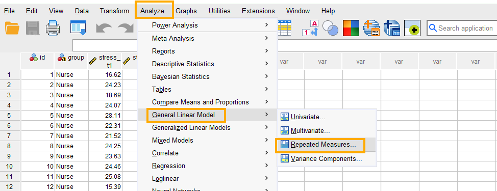
In SPSS, the two-way mixed repeated measures ANOVA test can be accessed from the menu Analyze / General Linear Model / Repeated Measures. So, as Figure 3 shows, we click on Analyze and then choose General Linear Model and then click on Repeated Measures.
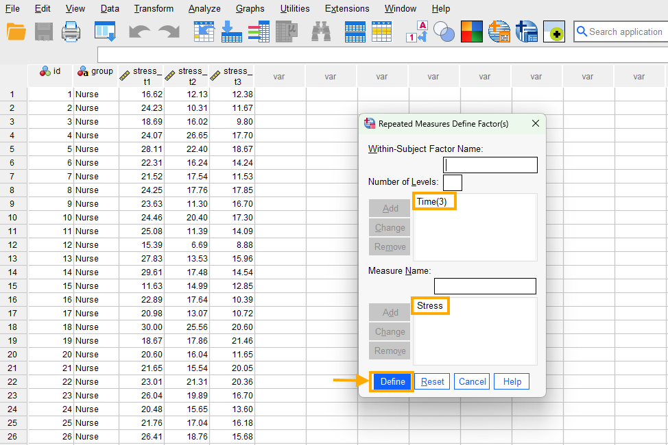
Once we click on Repeated Measures option, a window will pop out that asks for the name of Within-Subject Factor, the Number of Levels the factor has, and the name of the Measure (the dependent variable). Figure 4 shows the Repeated Measures Define Factor(s) window.
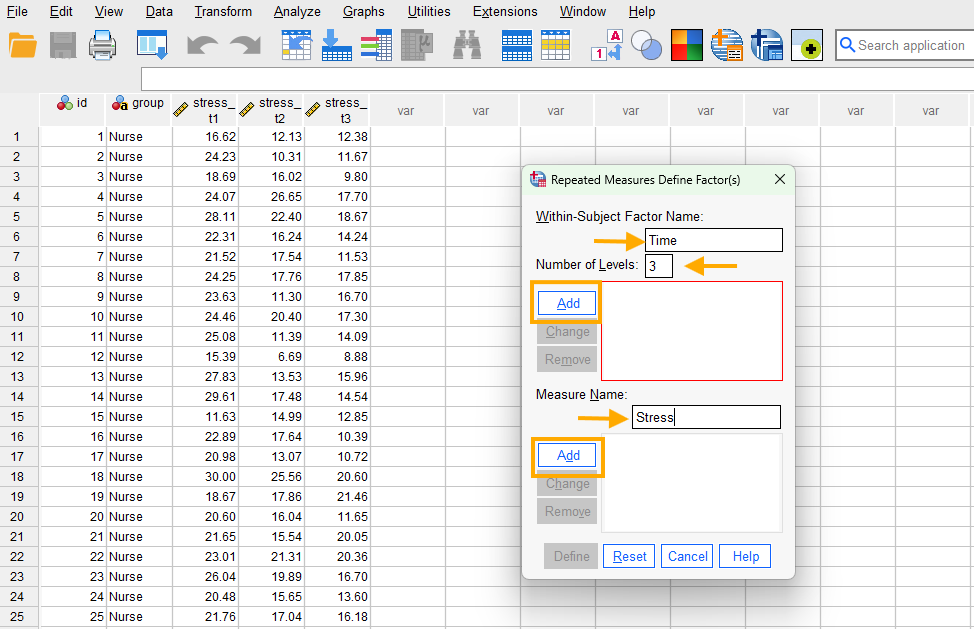
For Factor name, we choose Time, as the repeated measurements occurred over times. For the number of Levels, we enter 3 because we have three time points and measurements. We press Add button. For Measure Name, we choose the name Stress and press the Add button. Measure is synonymous with the dependent variable.
After defining the factor and the measure (dependent variable) name, the windows should look like Figure 5.
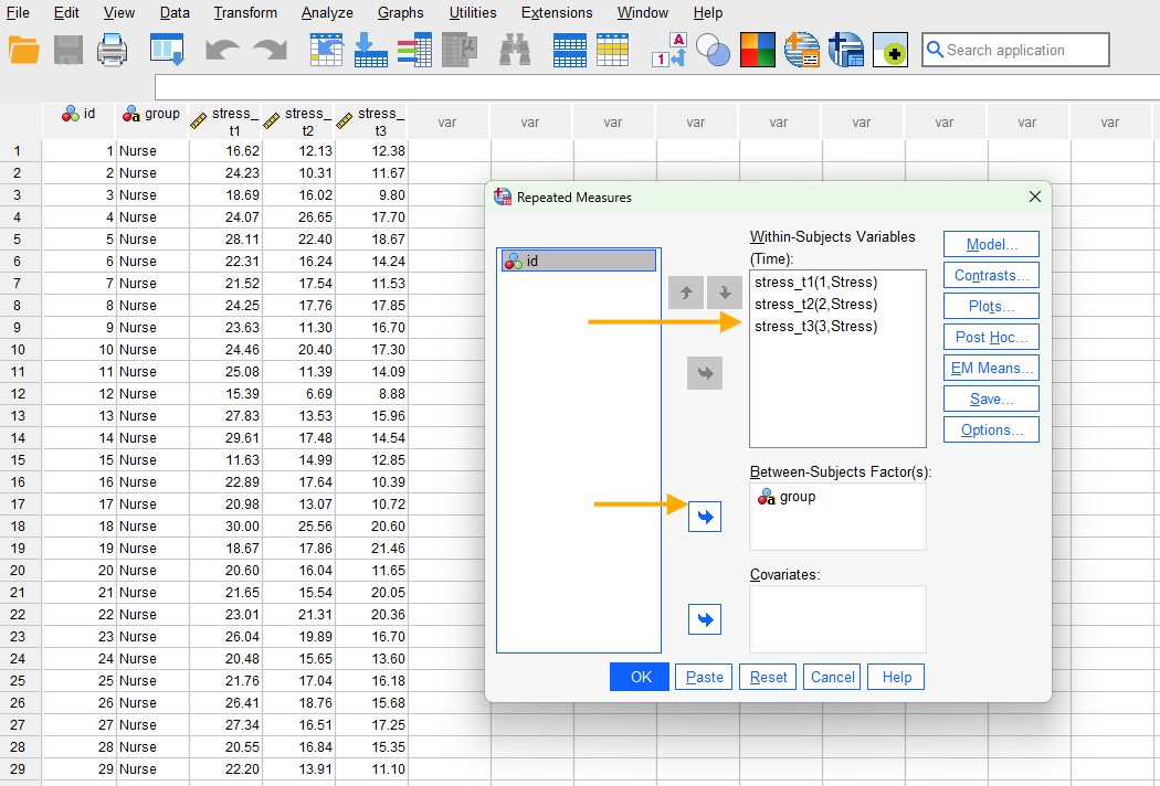
We then click on the Define button for defining the variables we just created. The previous window disappears and a new window (Figure 6) appears. In the new window (Figure 6), we can see our three Stress Time measures and in the opposite window we can see three slots with question marks and the numbers 1, 2, and 3. We pass each measurement level from the left panel into the corresponding slot in the opposite panel. We can click on the level name and use the blue right-arrow button to pass them to the right panel. After completing moving the levels to their respective time slots, the completed window should look like Figure 6 below.
While we are in the window, we can request for some additional results. If we want to plot the mean stress values for each group and across the three time points, we can click on Plots and ask for a plot for Time on the horizontal axis and separate lines for each group (Figure 7).
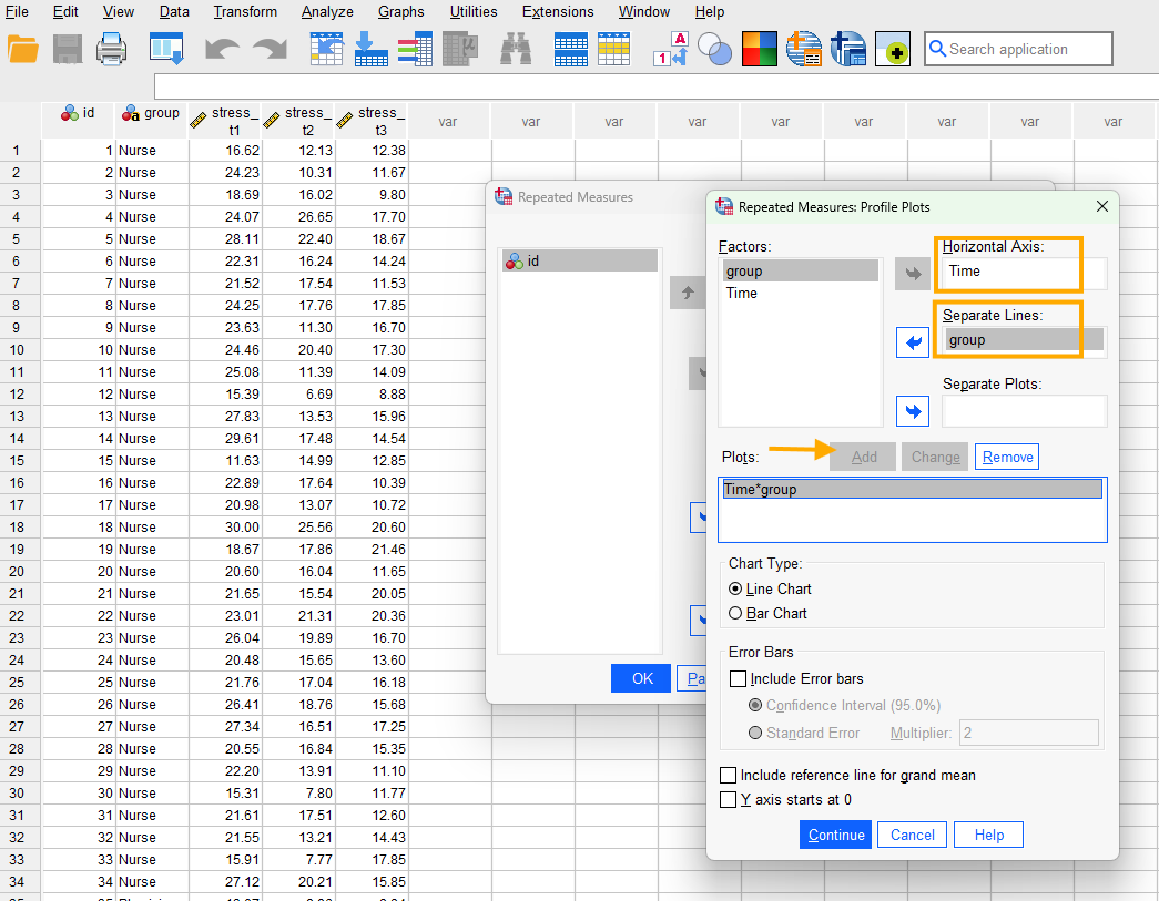
After entering Time into Horizontal Axis and group to Separate Lines box, we click on Add button. If you do not click on Add button and just click on Continue, no plot will be produced. We click on Continue (after Adding the plot) and close this window.
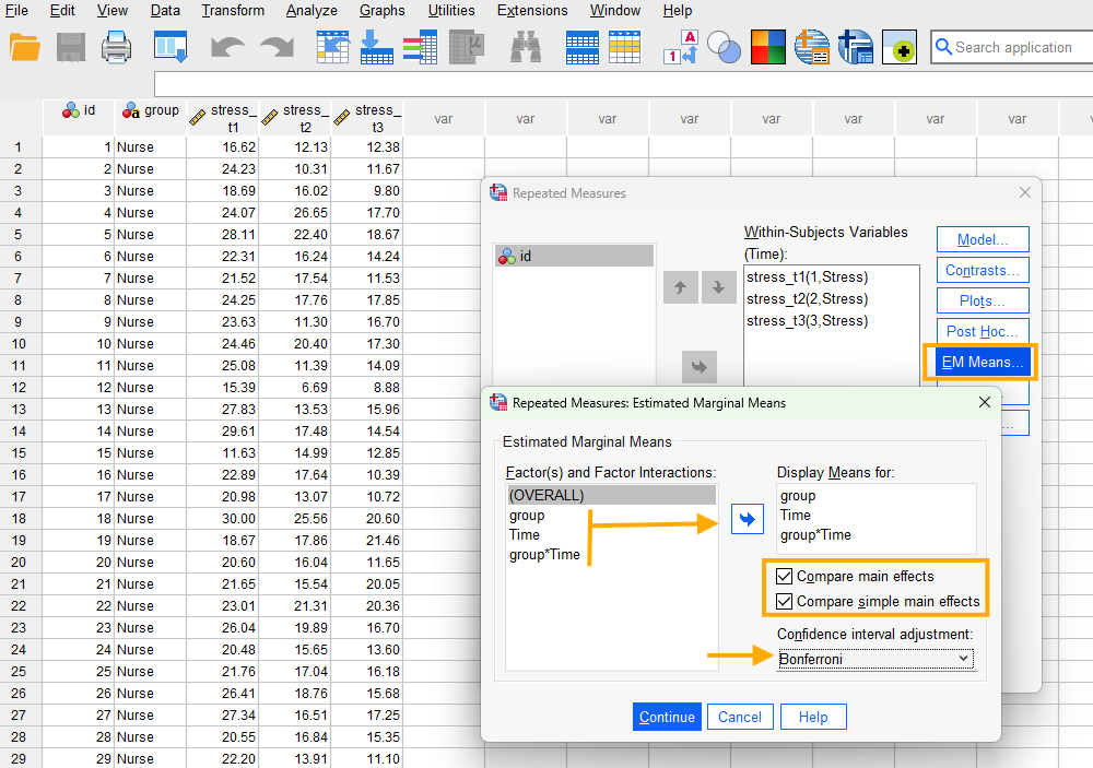
In the two-way mixed repeated measures ANOVA, we are also interested to know if the mean values are significantly different from each other between two groups, between time points, and the interaction of time by group. So, we click on the EM Means button and by selecting Time, Group, and Time*group (interaction term) from the left panel we move it to the Display Means for panel. Just below that tick Compare Main Effect and Compare simple main effects (for the interaction term) and from the menu below choose Bonferroni adjustment (Figure 8).
Next, we press Continue and then press the OK button to run the two-way mixed repeated measures ANOVA in SPSS.
Interpreting Two-way Mixed Repeated Measures ANOVA in SPSS
In this study, the researcher aims to evaluate the effectiveness of mindfulness program in reducing stress among hospital staff. In addition, the researcher is interested in knowing if the program has different effects on nurses and physicians. Since the same group of nurses and physicians participated in the study, the researcher employs a two-way mixed repeated measures ANOVA to compare the mean stress levels across the three time points and between nurses and physicians.
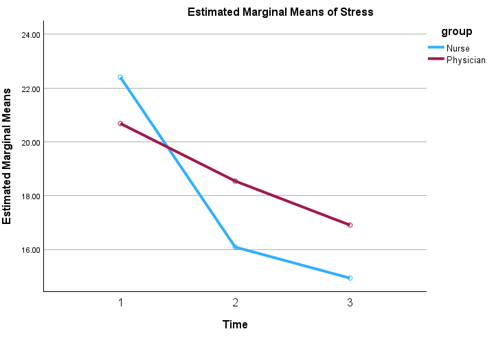
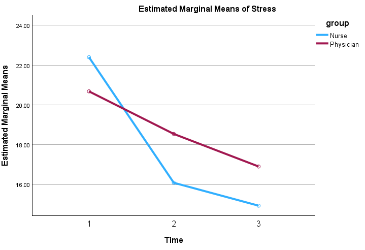
As Figure 9 above shows, the mean stress levels for both nurses and physicians show a decrease from Time 1 to Time 2 and from Time 2 to Time 3. We now go through the requested analysis results in the SPSS output one by one.
The first two tables (Figure 10) show the names of the levels of the dependent variable (Stress) and the size of each group.
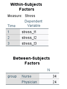
One point to note is that in this table, the three levels of the time correspond to three dependent variables under column Dependent Variable. Although we only have one dependent variable, SPSS regards the different measurements of stress at three time points as separate but related dependent variables. When a study has several related dependent variables, we call it multivariate analysis. Therefore, SPSS outputs several multivariate tests, as well.
The next table shows the Multivariate Tests. As we discussed above, SPSS considers the three measurements as three dependent variables and therefore produces several multivariate tests (Figure 11).
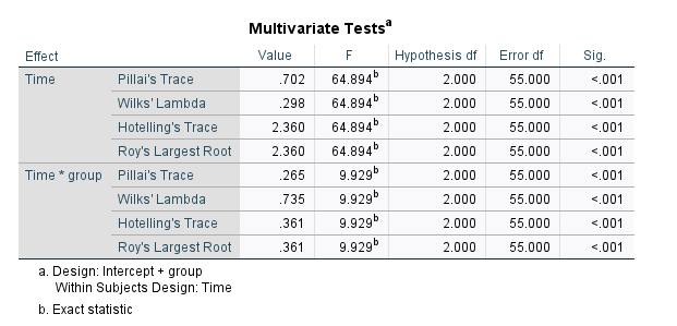
Although we can ignore this table, it hints at the statistical significance of our overall model (effect of time on three stress level scores) and the interaction between time and group. All four multivariate tests show that the overall model is statistically significant (p < 0.01).
The next table shows if the assumption of sphericity is met (Figure 12).
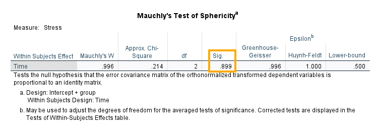
An assumption underlying the repeated measures ANOVA is the sphericity which means that the variances of difference scores (i.e., subtracting Time 2 from Time 1 scores, Time 3 from Time 1 scores, and Time 3 from Time 2 scores) are equal. The Mauchly’s test provides information if the variances are equal. As the results in Figure 13 show, the Mauchly’s W (0.996) is not statistically significant (p = 0.899), which means that the variances are not different. So, we assume the sphericity is met; otherwise, we should use other test results (shown in the next table).
In the next table (Figure 13), we can see the results of repeated measures ANOVA for both when sphericity is met and when sphericity is not met.
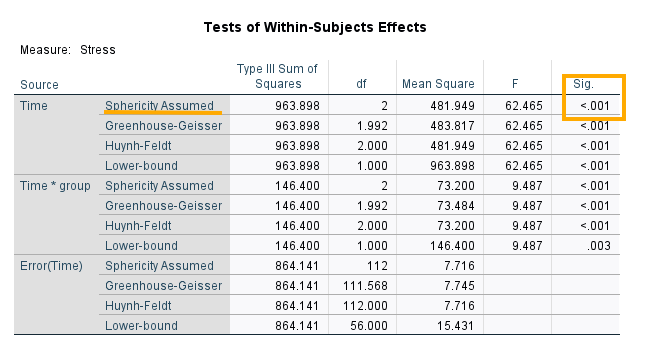
Because the sphericity assumption is met in this analysis, we can look at the first row (Sphericity Assumed) in the table to see the results of the repeated measures ANOVA. According to this table, the overall model is statistically significant with an F = 62.465 and p < 0.01. Therefore, we conclude that the overall change in mean stress level scores and the interaction between Time and Group is statistically significant.
The next table in the SPSS repeated measures ANOVA output is Tests of Within-Subjects Contrasts (Figure 14). This table shows if there is significant trend in measurement pattern (from Time 1 to Time 3), and if the trend is linear or quadratic. A trend test shows if the change (e.g., in stress levels) over different measurement times is significant or not.
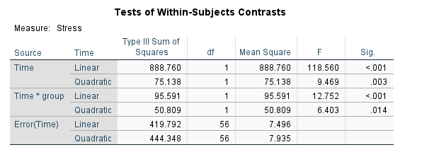
As we can see in Figure 14, both the linear trend and the quadratic trend are statistically significant. A significant linear trend demonstrates a strong monotonic change across time and a significant quadratic trend indicates that the middle time point differed from the average of the first and last time points (the trend analysis table is not usually reported in repeated measures ANOVA results.) Another table produced by SPSS output is Tests of Between-Subjects Effects (Figure 15).
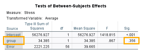
A between-subjects test is used if there is a grouping factor in the model (such as position role) and we want to know if that factor is statistically significant. In our example, the group included nurses and physicians (two groups). As the results show, at F = 0.867, the p-value is 0.356, which is not statistically significant. This means that the effect of the mindfulness program was equally effective on nurses and physicians.
As we discussed above, when the overall model is statistically significant, our next question would be which time points are statistically different from each other? The next set of tables (Figure 16) show the pairwise comparisons between nurses and physicians.
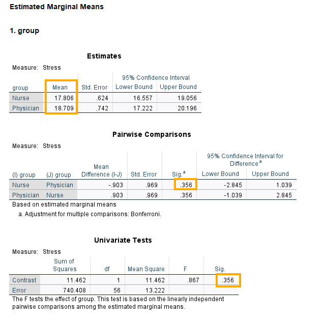
As we can see, the difference between the mean stress level (averaged across three time points) between nurses and the physicians is not statistically significant.
The next set of tables (Figure 17) show if the mindfulness program has a significant effect on the stress levels of combined group of nurses and physicians (disregarding group membership) on average and over different time points.
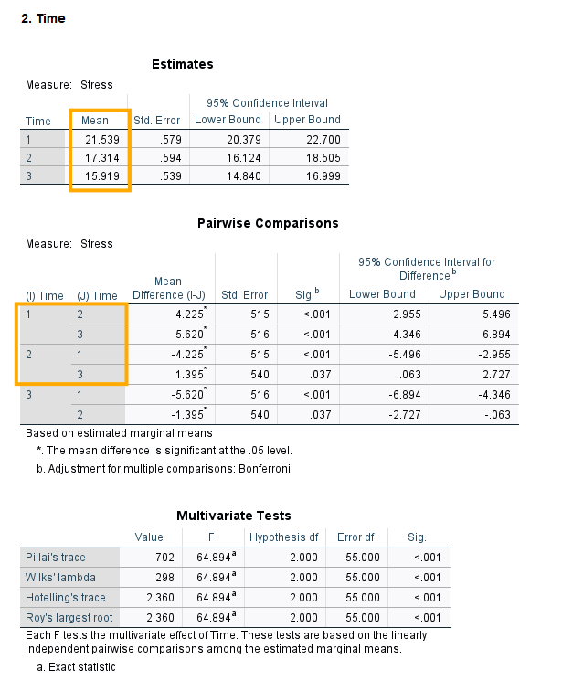
The Pairwise Comparison table compares the means of stress level scores in pairs:
- A comparison between Time 1 and Time 2 scores reveals a mean difference of 4.225, which is statistically significant (p < 0.01).
- A comparison between Time 1 and Time 3 scores reveals a mean difference of 5.620, which is statistically significant (p < 0.01).
- A comparison between Time 2 and Time 3 scores reveals a mean difference of 1.395, which is statistically significant (p = 0.037).
In summary, we conclude that after three months, the staff (nurses and physicians combined) stress levels significantly decreased. This shows the mindfulness program was effective even in three months into the program. But was it equally effective for both nurses and physicians? We can look at the interaction (group * Time) set of tables below (Figure 18).
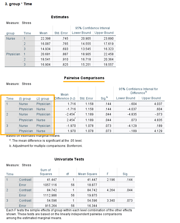
The Pairwise Comparisons table shows the difference between nurses and physicians at each time point. At time 1, the difference is not significant (p = 0.144). This shows that the baseline measurement was similar between nurses and physicians. At time 2, the difference was significant (p = 0.044), but marginally. At time 3, the difference was not significant (p = 0.073). These results support the Between-Subjects tests above, that showed no significant difference between nurses and physicians overall.
The next series of tables (Figure 19) show the simple effects of the treatment at each time point separately for nurses and physicians.
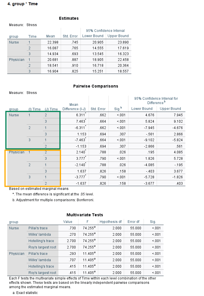
In the Pairwise Comparisons table, we can see that the stress level among nurses changed significantly from Time 1 to Time 2 (p < 0.001) and from Time 1 to Time 3 (p < 0.001), but not significantly from Time 2 to Time 3 (p = 0.307). Similar pattern can be seen among the physicians group.
Figure 20 shows the estimated mean stress levels at times 1, 2, and 3 for nurses and physicians. The crossing lines indicate an interaction between Time and Group.
Reporting Two-way Mixed Repeated Measures ANOVA Results
In this study, the focus was on evaluating the effectiveness of a mindfulness program in reducing stress levels among nurses and physicians at a hospital. A random sample of 34 nurses and 24 physicians were selected, and their stress levels were assessed at three distinct time points: Time 1 (program initiation), Time 2 (three months into the program), and Time 3 (six months into the program). Stress level was measured using a valid and reliable questionnaire.
A two-way mixed repeated measures ANOVA was conducted to compare the mean stress scores across the three time points and between the two groups (nurses and physicians). The Mauchly test showed that the sphericity assumption was met (W = 0.996, p = 0.899). The within-subjects results showed a significant effect of time on stress levels (F(2, 48) = 62.47, p < 0.01, indicating that stress decreased significantly over time. However, the between-subjects tests showed no statistical difference between nurses and physicians on their mean stress levels when stress scores were averaged across all time points.
These results suggest that the mindfulness program significantly reduced stress among hospital staff comparably benefiting both groups, though nurses showed a larger reduction.