SPSS FOCUS
A comprehensive guide to statistical analysis in SPSS
Multiple Regression in SPSS
Multiple regression is a statistical method that measures and models the relationship between two or more independent variables and one continuous dependent variable. The independent variables can be continuous, binary, or categorical. Modeling in multiple regression involves obtaining an equation from data that incorporates multiple predictors to better explain or predict a future outcome. Multiple regression is a fundamental method in predictive modeling, often used when the dependent variable is influenced by multiple factors simultaneously.
Introduction to Multiple Regression
We learned about regression in the simple linear regression module. A simple linear regression is used to model the relationship between one independent variable and the dependent variable. Such a simple linear regression could provide an acceptable fitted model to explain the relationship between the independent variable and the dependent variable (for example, by looking at the value of the R²). However, a single independent variable may not provide enough information to predict the dependent variable and may leave some unexplained variance in the dependent variable.
One way to add more information and reduce the unexplained variance in the dependent variable is to add more relevant independent variables based on theory, prior research, or expert opinion. For example, exercise may be a good predictor of weight loss, but including diet type can also contribute to predicting weight loss. In other words, instead of a simple linear regression, we can use multiple linear regression to evaluate independent variables that predict weight loss.
Like a simple linear regression, the dependent variable in a multiple linear regression is continuous (measured on an interval or a ratio scale of measurement). However, the independent variables can be continuous, binary (two levels, like sex: male and female), or categorical (more than two levels, such as income: low income, middle income, and high income).
In multiple linear regression, one assumption is that the independent variables (predictors) are not highly correlated with each other. If the independent variables are highly correlated, the estimated regression coefficients will be unstable due to inflated variance. In addition, because of the high correlation of the independent variables, we cannot exactly infer the effect of the individual independent variables. The problem of highly correlated independent variables in multiple regression is called multicollinearity or collinearity problem. Therefore, we must make sure our independent variables are not highly correlated with each other. We can test for the existence of multicollinearity problem using correlation tests among independent variables, or use an index called variance inflation factor (VIF).
In the following sections, we present an example research scenario where a multiple regression will be used to analyze the data and predict an outcome. We will demonstrate how to perform a multiple regression in the SPSS program step-by-step and how to interpret multiple regression analysis results in the SPSS output.
Multiple Regression Example
What is the relationship between the number of hours students study, students’ academic motivation, and their test scores? Can the number of study hours and academic motivation predict students’ test scores?

Photo courtesy: Jerry Wang, Unsplash
A schoolteacher is interested in modeling the relationship between the number of hours students study and their academic motivation and the scores the students achieve on a test. The teacher randomly selects 65 students from the school district and asks the students how much time they dedicated to preparing for the test. In addition, the teacher administers a questionnaire on school motivation to understand how motivated the students are for their studies. The teacher is not only interested in understanding the relationship between study hours and academic motivation and test scores, but also if the number of study hours and the motivation of students can be used to predict a student’s test score.
Table 1 shows the scores of five students on the test (dependent variable) along with the number of weekly hours they studied and their motivation score on 0-100 scale (two independent variables).
| Student | Study Hours | Motivation Score | Test Score |
|---|---|---|---|
| Student 1 | 35 | 74 | 84 |
| Student 2 | 37 | 69 | 81 |
| Student 3 | 32 | 47 | 58 |
| Student 4 | 39 | 63 | 80 |
| Student 5 | 46 | 56 | 85 |
| … | … | … | … |
The teacher enters the data in the SPSS program in the computer lab. The data for this example can be downloaded in the SPSS format or in CSV format.
Entering Data into SPSS
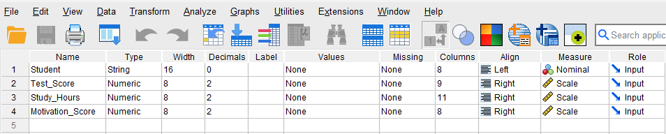
To enter the data in the SPSS program, first we click on the Variable View tab (bottom left) and create these four variables under name column: Student, Study hours, Motivation score, and Test score. We specify the following attributes for each variable:
- Student: Type is string. Width is 16. Measure is Nominal.
- Study_Hours: Type is Numeric. Measure is Scale.
- Motivation_Score: Type is Numeric. Measure is Scale.
- Test_Score: Type is Numeric. Measure is Scale.
When defining the variables, we specify both the data type and the measurement level for SPSS. The data type is used by the SPSS software to understand the data type (e.g., text, numbers, dates, etc.), while the measurement level helps the statistical algorithm for running the appropriate analysis.
In our data, the Student variable consists of student names or IDs and is not included in the computation; therefore, we select “String” as the data type and “Nominal” (i.e., not a number) as the measurement level. For the three continuous variables (Study_Hours, Motivation_Score, and Test_Score) we choose Numeric for their data types and Scale for their measurement levels. SPSS uses the term scale for both interval and ratio measurement levels. After creating all variables, the Variable View panel of SPSS for our dataset should look like Figure 1.
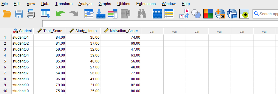
Once the variables are created, we can enter the data into the columns Student, Study_Hours, Motivation_Score, and Test_Score in the Data View tab of SPSS program. For Student, we can enter their names or an ID. For the variable Study_Hours, we enter the number of hours each student reports studying. For the Motivation_Score, we enter the students’ scores on the motivation questionnaire. Finally, we enter the test scores in Test_Score column for each student. Figure 2 shows how the data for all three variables should look like in the Data View tab.
Now we are ready to conduct a multiple regression analysis in SPSS!
Analysis: Multiple Regression in SPSS
Multiple regression is a statistical modeling method for modeling the relationship between two or more independent variables and one dependent variable for the purpose of predicting future values and understanding the direction, strength, and significance of the conditional relationship between the independent variables and a dependent variable.
In our example research study, a teacher is interested in modeling the relationship between the number of weekly hours students spend studying and their academic motivation (our two independent variables) with students’ test scores (the dependent variable). To investigate this relationship, the teacher collects data on the study hours and school motivation and test scores from a random sample of 65 students. The teacher uses the multiple regression method because there are two independent variables and one continuous dependent variable.
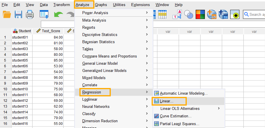
In SPSS, multiple linear regression can be accessed through the menu Analyze / Regression / Linear. So, as Figure 3 shows, we click on Analyze and then choose Regression and then Linear.
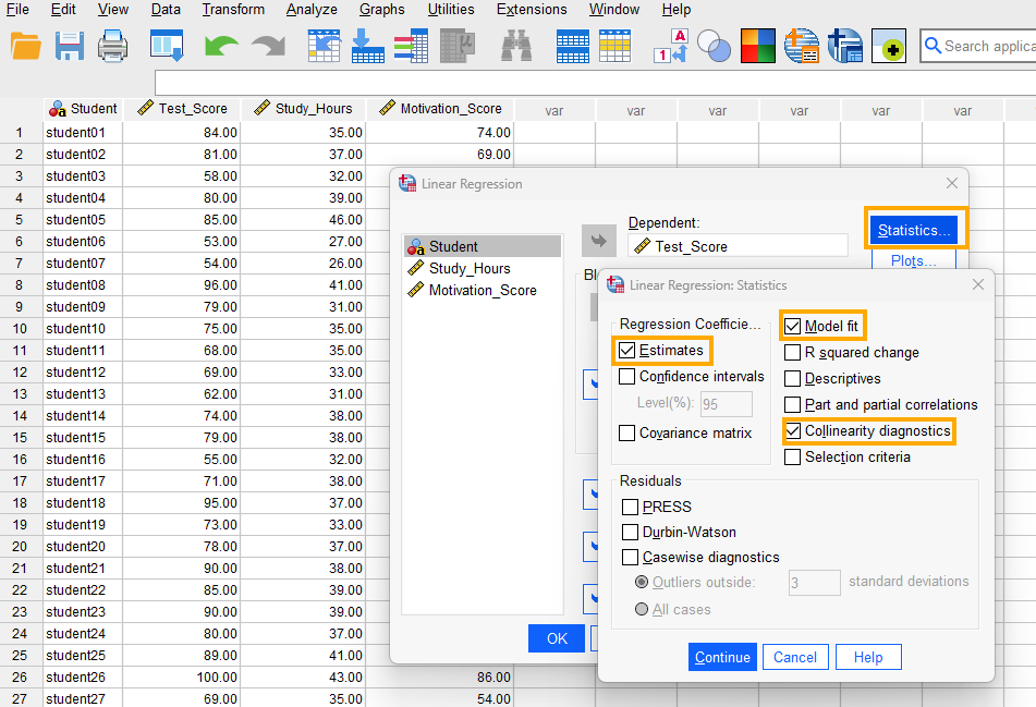
After clicking on Linear, a window will appear asking for Dependent and Independent(s) variables we want to model using multiple regression (Figure 4). We send Test_Score into the Dependent box and Study_Hours and Motivation_Score into the Independent(s) box.
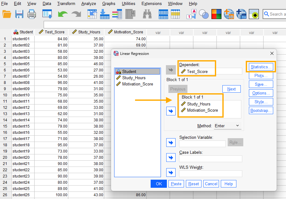
In addition, because we want to make sure the two independent variables are unrelated, we request collinearity diagnostics (such as tolerance and variance inflation factor, VIF). Collinearity (or multicolliearity) issue occurs when the predictor variables in a multiple regression model are highly correlated and therefore may absorb each other’s variance and effect, so that we are not sure if the effect is related to that predictor or the correlated predictor. So, we click on Statistics button and select Estimates, Model fit, and Collinearity diagnostics options (Figure 5).
Finally, we click on Continue and OK to run the multiple regression analysis. SPSS will produce the results of the multiple regression analysis in the Output window.
Interpreting Multiple Regression in SPSS
In our example research study, a teacher is interested in investigating the relationship between the number of weekly hours students spend studying and their academic motivation with their test scores. In this example, the dependent variable is the students’ test scores and the independent variables (the predictors) are the number of weekly study hours and motivation scores. The teacher runs a multiple regression in SPSS and gets several tables in the Output file.
The first table in the output (Figure 6) shows the names of the independent and dependent variables analyzed by multiple regression.
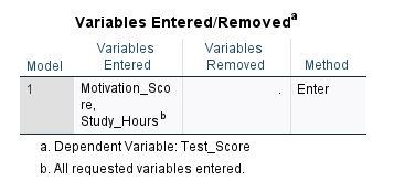
As Figure 5 shows, there are two independent variables entered into our model: Study hours and Motivation score, with Test score as our dependent variable.
The next table, the Model Summary table (Figure 7), shows the relationship between Study hours and Test scores using R, R Square, and Adjusted R Square statistics.
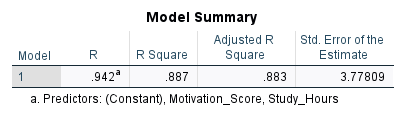
The R statistic is the multiple correlation coefficient measured between the combination of Study hours and Motivation score with the Test scores. Multiple correlation is calculated as the Pearson correlation between the predicted values and the actual observed values and varies between 0 and 1 (unlike Pearson correlation coefficient, which varies between -1 and 1). As we stated in the introduction, besides predictive modeling, a regression analysis can also show the relationship (and direction and significance of the relationship) between variables. In our example, the combined correlation between Study hours and Motivation score with Test scores is 0.942, which is relatively high.
The R Square (0.887) statistic shows the amount of variance in the dependent variable explained by the independent variable(s). In other words, R Square shows how much information the independent variables bring to our model (and how much is left out). The higher the R Square, the more informative the independent variables are. The R Square values can also be used to compare different regression models to understand which model better explains the variability in the outcome variable.
Adjusted R Square takes into account factors that inflate R Square, such as the number of independent variables. So, we recommend looking at Adjusted R Square as a more unbiased measure of the informativeness of our independent variables. In this example, the adjusted R Square is 0.883, implying that the linear combination of Study hours and Motivation score can explain about 88% of the variance in the dependent variable in the model while about 12% of variance (1 – 0.88 = 0.12) remains unaccounted for (we do not know the source of variance).
Next, the ANOVA table (Figure 8) looks at regression from an analysis of variance perspective where different forms of variances (sum of squares) are reported.
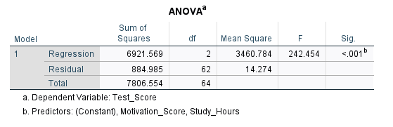
The ANOVA table provides two sources of variance and calls them Sum of Squares: Regression sum of squares and Residual sum of square. The Regression part shows the information, and the Residual part shows noise or unknown information. We want a high information to noise ratio (also known as signal to noise ratio). The higher this ratio, the more likely our model will be statistically significant and meaningful. In this ANOVA table, we can see that F = 242.454 and is statistically significant (p < 0.05). So, our regression model is statistically significant. The F value is calculated as the ratio of mean sum of squares of the regression to residual values (3460.784 / 14.274 = 242.454).
The statistics needed to interpret the relationship between Study hours and Motivation with Test scores are presented in the Coefficients table (Figure 9).
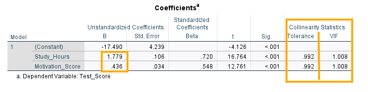
There are three rows in the table: Constant, Study hours, and Motivation score, each with a coefficient B value (-17.490, 1.779, 0.436, respectively). The B values are the coefficients of the regression model and come in two versions: unstandardized and standardized. The unstandardized version is on the original scale of the independent variable while the standardized version has been scaled to vary between -1 and 1.
In this table, Constant is the intercept, which is the point on the Z axis (the dependent variable) when the regression plane passes through (where the independent variables equal 0). In our example, the intercept is -17.490, meaning that when Study hours is zero and Motivation is totally absent, we theoretically expect the test score to be -17.490 on average.
The next two rows in the Coefficients table show the coefficients for (effects of) the two independent variables Study hours and Motivation , which are 1.779 and 0.436, respectively, and which are both positive and statistically significant (p < 0.01).
The last two columns in the Coefficients table (Figure 9 above) are the collinearity statistics. Tolerance and variance inflation factor (VIF) are common indices for checking collinearity. For tolerance, a value close to 1 and larger than 0.20 show weak collinearity. For VIF, values less than 10 show weak collinearity. We can see that for our set of predictors tolerance is close to 1 and VIF is 1.008. Therefore, we conclude that collinearity is not an issue in our model and variances are not inflated. SPSS additionally produces a separate collinearity diagnostics table (Figure 10) based on latent dimensions.
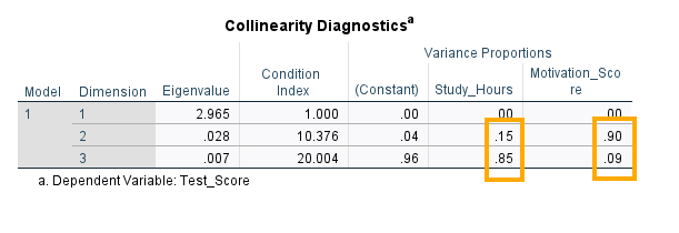
In Figure 10, there are three dimensions and three variables: constant, study hours, and motivation score. We look for the same dimension where both predictors have large variance proportions. In Dimension 2, Constant = .04, Study hours = .15 (small), and Motivation score = .90 (large). Only Motivation score loads heavily here; Study hours does not. In Dimension 3, Constant) = .96 (large), Study hours = .85 (large), and Motivation score = .09 (small). Study hours and the constant load heavily here; Motivation score does not. There is no dimension where both Study hours and Motivation score simultaneously have large variance proportions. That means these two predictors are not strongly collinear with each other.
Now that we have regression model coefficients, we can build our model. We can write the result of the analysis from the Coefficient table above in terms of the relationship between the test score and the linear combination of Study hours and Motivation as the following equation (model):
Predicted Test Score = -17.490 + 1.779 * Study_Hours + 0.436 * Motivation
In a multiple linear regression, individual coefficients for an independent variable are interpreted with regard to the other independent variables in the final model. For example, the coefficient (effect) for the Study hours is interpreted as follows: for each additional hour of study, the test score increases on average 1.779 score controlling for the Motivation variable. By controlling for motivation we mean keeping the Motivation variable at a fixed value and changing the study hours value freely. We demonstrate this concept in the following equation. According to the results from the multiple linear regression example,
Predicted Test Score = -17.490 + 1.779 * Study hours + 0.436 * Motivation
The equation above is our model and we can use it to predict a test score if we have information about the number of study hours and motivation. For example, if an student studies 40 hours a week and whose motivation score is 86, we predict their test score to be:
Predicted Test Score = -17.490 + 1.779 *(40) + 0.436*(86) = 91.166
Now let’s explore what we mean by “for each additional hour of study, the test score increases on average 1.778 scores controlling for the Motivation variable.” In the example above, Study hours value was set to 40. Now, for each additional hour of study, such as one hour, the test score increases on average 1.778 scores controlling for motivation. And we said “controlling for” means fixing the other variable at a constant value, such as 86 in example above. Let’s calculate the new score for one additional hour of study (from 40 hours to 41 hours) but given the same motivation value (86):
Predicted Test Score = -17.490 + 1.779 *(41) + 0.436*(86) = 92.945
We can see that the test score increased to 92.945 for one additional hour of study and keeping the motivation unchanged (controlled for). The increase in score is: 92.945 – 91.166 = 1.779, which is the coefficient of the Study hours variable in the SPSS results. We can reason the same for one unit change in Motivation, controlling for Study hours, which increases the test score by 0.436.
Reporting Multiple Regression Results
In this research, we aimed to explore the relationship between the number of hours students dedicate to studying and their academic motivation with their test scores. To investigate this question, we selected a random sample of 65 students and collected data on the hours students spent studying, their motivation scores from a reliable and valid questionnaire, and their test scores.
The results of the multiple regression analysis revealed that both study hours and motivation significantly influence test scores (F = 242.454, p < 0.05). The adjusted coefficient of determination, R²=0.883, shows that approximately 88% of the variation in test scores is explained by study hours and academic motivation. This suggests a strong relationship, emphasizing the impact of dedicated study time and academic motivation on school performance.
These findings underline the importance of consistent study habits in achieving higher test scores and encouragement from parents, teachers, and other stakeholders in a student’s education. These insights offer valuable guidance for both students and educators, demonstrating the significance of strategic time management and motivation in enhancing academic outcomes.