SPSS FOCUS

Measures of central tendency are values derived from a distribution that describe its typical or most common point. In other words, they indicate the value around which the other data points cluster. These measures provide a concise summary of the overall distribution. The most common measures of central tendency are the mean, median, and mode. In research papers, they are typically reported in the descriptive or exploratory statistics section—often in a table commonly referred to as Table 1.

When our data is measured on a ratio or interval (continuous) scale, the mean is one of the most useful piece of summary information about the distribution of our data. The mean is also known as the average or the arithmetic mean or the expected value. The mean is calculated by adding the values of a variable (distribution) and dividing the sum by the number of values:

For example, a researcher has collected the following blood pressure measurements from five patients: [132, 137, 163, 141, 141]. The mean blood pressure is

The mean value is an informative summary statistic if there are no extreme values in the distribution because those extreme values distort the mean value as a representative of the central tendency. Extreme values pull the mean value away from its central position, especially in small samples. In such cases, we should report the median.

Another measure of central tendency is the median of the distribution, which is the value in the data distribution that divides the sorted distribution into two equal halves. In other words, 50% of the values are below the median, and 50% are above the median. For this reason, median is also referred to as the 50th percentile ($P_{50}$). The median is an informative summary statistic if the distribution of data has extreme values in it or the distribution is not symmetrical. For example, in reporting housing property values, the median property value is commonly reported because of presence of property values that are much higher than the typical house.

The median of a data distribution can be located by first sorting the data from smallest to the greatest, and then finding the middle value (for odd number of data points). If there are an even number of data points (e.g., 10 blood pressures measurements), the median is defined to be the average of the two middle values (i.e., the average of the fifth and the sixth ordered values). For example, for the following 11 blood pressure measurements [132, 137, 163, 141, 141, 142, 166, 147, 121, 130, 133], first we sort them: [121, 130, 132, 133, 137, 141, 141, 142, 147, 163, 166], and find the middle value as the median, which is 141.

For the following sorted 10 blood pressure measurements, [121, 130, 132, 133, 137, 141, 141, 142, 147, 163], since there are even (10) numbers, the median is the average of the 5th and 6th values: (137 + 141) / 2 = 139.

In a data distribution, some values may repeat several times. The value with the highest repetition (frequency or occurrence) is the mode of the distribution. For example, in a distribution of blood pressure measurements, the value 142 could be the most repeated (most frequent). In a questionnaire, respondents may choose an option more frequently than other options, revealing a mode. If a distribution has two values with equal number of repetitions, that distribution is referred to as bimodal. For example, if blood pressure measurement 142 is repeated seven times and blood pressure 130 is also repeated seven times, the distribution has two modes and is characterized as a bimodal distribution.

Calculating the measures of central tendency (the mean, the median, and the mode) is possible in the data exploration menus of SPSS. We demonstrate how the mean, the median, and the mode of a variable (measures of central tendency) are calculated using blood pressure measurement dataset. The dataset can be download as SPSS format or CSV format from this link. The data includes blood pressure measurements of 30 patients at two time points (BP01 and BP02). Once downloaded, we open the data file in SPSS. We are interested in knowing the mean, the median, and the mode of blood pressure measurements at time 1 (BP01).

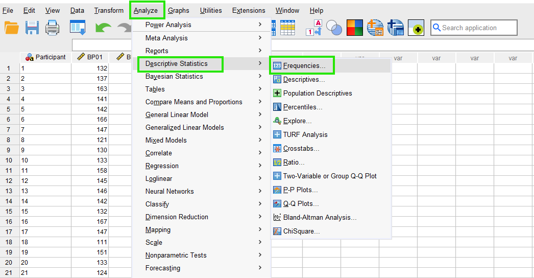
In SPSS, measures of central tendency can be accessed together through the menu Analyze / Descriptive Statistics / Frequencies. So, as Figure 1 shows, we click on Analyze and then choose Descriptive Statistics and then Frequencies.

Once we click on Frequencies, a new window will pop out asking for the variable name (BP01). So, we send BP01 to the Variables box (Figure 2).

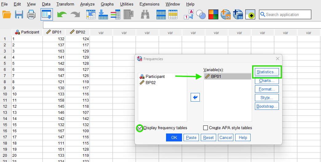
While still in this window, we tick the option Display frequency tables and then click on Statistics button to choose measures of central tendency (Figure 3).

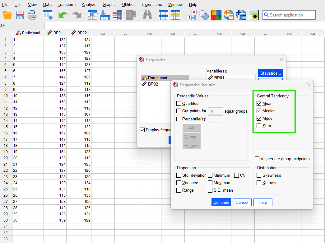
In the Statistics window, under Central Tendency, we tick the boxes for Mean, Median, and Mode and click on Continue and finally on OK buttons. The SPSS output shows the results for the selected measures of central tendency in two tables.

The first table (titled Statistics, Figure 4) returns the values for the mean, median, and the mode of the blood pressure measurements data.

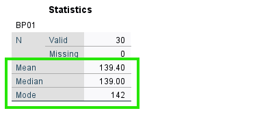
According to the Statistics table, the mean = 139.40, the median = 139.00, and the mode = 142. As we described above, median is preferred to the mean if the data distribution includes extreme values. However, it seems in this variable, the mean and median are very similar, hence we can report the mean.

The mode is the value which has the highest occurrence or frequency. The table in Figure 5 shows the frequency of each unique value.

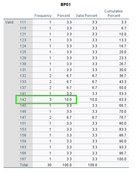
We can find the mode by locating the value with the highest frequency or absolute percentage. In this table, we can see that the value 142 has the highest frequency (3) and the highest absolute percentage (10%). Therefore, SPSS has selected the value 142 as the mode of the distribution (as reported in the Statistics table).