SPSS FOCUS
A comprehensive guide to statistical analysis in SPSS
ANCOVA in SPSS
ANCOVA (analysis of covariance) is a widely used statistical method for comparing the mean values of several groups on a continuous outcome considering the effect of a related continuous variable on the outcome. ANCOVA extends ANOVA (analysis of variance) by including a continuous independent variable in the model to reduce bias and confounding effect hypothetically caused by that additional variable (called controlling variable or covariate). ANCOVA can be performed in both an ANOVA framework and in linear modeling framework (e.g., multiple regression).
Introduction to ANCOVA
When it comes to comparing the means between two or more than two groups, several statistical methods are available to analyze the data, such as t-tests, ANOVA, or regression models. For example, a researcher may be interested in investigating the treatment effect of two medications on blood pressure. The researcher could use a t-test to see if the mean differences between the groups receiving the two medications are statistically and clinically significant. However, the differences observed between the two groups could be in part due to another factor, such as the initial blood pressure of the participants, their BMI, or other confounding variables, making the results biased.
One remedy to reducing bias and within-group error variance in observational or quasi-experimental data is to include controlling variables (covariates) that are assumed to influence the outcome. In other words, there may be some independent variables other than the main factors in the experiment or study that have a correlation with the outcome of interest (e.g., the treatment effect). In this case, statistical methods, such as analysis of covariance (ANCOVA), should be used to adjust the outcome measurements for the presence of influential covariates. After adjusting for a covariate, the outcome measurements may change.
ANCOVA can be viewed as an extension of ANOVA that incorporates an extra continuous covariate believed to have confounding influence on the relationship between the research variables. Similar to ANOVA, the results from an ANCOVA analysis allow us to compare the means between two or more than two groups after adjusting for (or controlling for) the confounding variable. In other words, ANCOVA removes the variance due to the confounding variable and also the within-group error variance. Once an ANCOVA test is statistically significant, post hoc or contrast tests (such as Bonferroni) can be performed to find which group means differ statistically significantly from each other after controlling for the covariates.
Similar to an ANOVA test, an ANCOVA test requires some assumptions to be met, such as,
- Linearity — The covariate must have a linear relationship with the dependent variable.
- Homogeneity of regression slopes — The covariate–outcome relationship must be the same across all groups (tested via the group × covariate interaction).
- Independence of the covariate and treatment — The covariate must be measured before treatment and must not be affected by it.
- Normality and homoscedasticity of residuals — Standard linear model assumptions apply.
The assumption of homogeneity of regression slopes (lack of significant interaction between the group and the covariate) must be investigated before running ANCOVA. In the following sections, we present an example research scenario where a one-way ANCOVA test will be used to analyze the data. We will demonstrate how to perform ANCOVA in SPSS step-by-step and how to interpret the SPSS results.
ANCOVA Example
Is there a difference between female and male high jump athletes in their jump performance? Is there a difference after taking into account the athletes’ heights?

A sports scientist is interested in understanding whether male and female high jump athletes differ in their jump performance, and whether any observed gender differences remain after accounting for athletes’ height.
High jump performance depends on biomechanical and physiological factors such as strength, technique, and body structure. Height may provide a mechanical advantage in high jump events, and male athletes are, on average, taller than female athletes. Therefore, apparent gender differences in performance may be partly explained by differences in height rather than gender itself.
The sports scientist decides to verify this hypothesis using data collected from female and male athletes from a high school. The researcher collects data on how high the athletes have jumped (in centimeters), their gender (female, male), and their heights (in centimeters). Table 1 shows the data for five athletes.
| Sex | Height (cm) | Jump (cm) |
|---|---|---|
| Female | 161.6 | 108.5 |
| Female | 163.6 | 134.3 |
| Male | 176.5 | 126.9 |
| Male | 170.8 | 121.7 |
| Female | 174.4 | 136.7 |
| … | … | … |
In this study, the sports scientist is interested to know if female and male athletes differ in their jump performance. In addition, the sports scientist is curious to know if taking into account the heights of the athletes would change the results observed. Therefore, the sports researcher, after collecting the data and checking for the required assumptions, decides to run an analysis of variance (one-way ANOVA) to compare female and male athletes on their jump performance. For controlling the athletes’ heights, the sports scientist decides to use analysis of covariance (ANCOVA) by adding the athletes’ height as a covariate. The data for this example can be downloaded in the SPSS format or in the CSV format.
Entering Data into SPSS
To enter the data in the SPSS program, first we click on the Variable View tab (bottom left) and create four variables under name: ID, sex, height_cm, jump_cm. We specify the following attributes for each variable:
- ID: Type is string. Width is 8. Measure is Nominal.
- sex: Type is Numeric. Measure is Nominal.
- height_cm: Type is Numeric. Measurement is Scale.
- jump_cm: Type is Numeric. Measurement is Scale
When defining the variables, we must specify both the data type and the measurement level for SPSS. The data type is used by the program to read the data, while the measurement level is used by the statistical algorithm for computation.
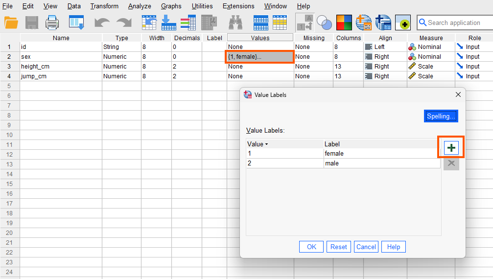
For the sex variable, although the values are labels (female and male), we assign numbers to them. So, we choose “Numeric” as the data type but select “Nominal” as the measurement level. To assign numbers to sex labels, in the Value column, click on the cell in the sex row to open a window. In the Value box, enter 1 and in the Label box, enter “female,” then click “add.” Repeat this process with Value 2 for the “male” and close the window. Figure 1 shows how to create sex levels (female, male) and assign numbers to them.
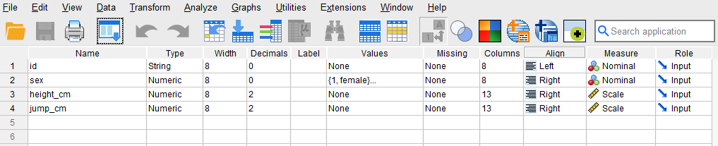
The data type for the variables height_cm and jump_cm are “Numeric,” and for the measurement level, we select “Scale.” After creating all variables, the Variable View panel of SPSS for our dataset should look like Figure 2.
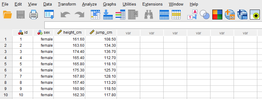
Once the variables are created, we can enter the data into the columns ID, sex, height_cm, and jump_cm in the Data View tab of SPSS program. For ID, we can enter names or an ID. For the variable sex, we can either directly type the sex directly (female or male), or the values we assigned them during the variable creation step in the Variable View tab (1 = female, 2 = male). Next, we enter the athletes’ height in column height_cm and how high they jumped in jump_cm column. Figure 3 shows how the data for all three variables should look like in the Data View tab.
Now we are ready to run the ANCOVA in SPSS!
Analysis: ANCOVA in SPSS
ANCOVA is a statistical method that is used to compare the conditional means of several groups adjusting for a covariate. The inclusion of a covariate is based on the hypothesis that the covariate is correlated with the outcome / dependent variable and therefore must be taken into account when studying the effect of a factor on the outcome. In the present study, the researcher is interested in understanding if the performance of female and male athletes in high jump is different and if such a difference persists after taking into consideration the heights of the athletes. Therefore, the researcher conducts an ANCOVA in which the heights of the athletes are entered the model as a covariate.
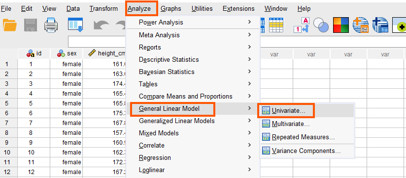
ANCOVA in SPSS can be accessed from the menu Analyze / General Linear Model / Univariate. So, as Figure 4 shows, we click on Analyze and then choose General Linear Models and then Univariate.
After clicking on Univariate, a window will appear asking for Dependent Variable, Fixed Factor(s) (i.e., independent variables), and the Covariate(s). We send jump_cm into the Dependent Variable box, and the sex into the Factor(s) box, and the height_cm into the Covariate(s) box. Figure 5 shows how the window should be populated with our dependent, covariate, and the independent variables.
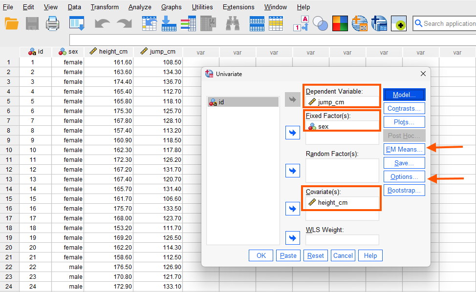
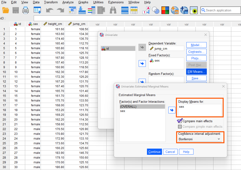
While in this window, we also choose to calculate conditional mean by clicking on EM Means and unconditional means by clicking on Options. Figure 6 shows the EM Means window. We send sex into Display Means for box. Optionally, we can choose Compare main effects and choose Bonferroni adjustment. This is optional because we only have two groups and therefore, we do not need Bonferroni adjustment. However, if we had three or more groups, and if the overall model was statistically significant, we could use Bonferroni adjustment for pairwise comparison controlling for familywise error.
We click on Continue and next click on Options button. Another window will appear (Figure 7).
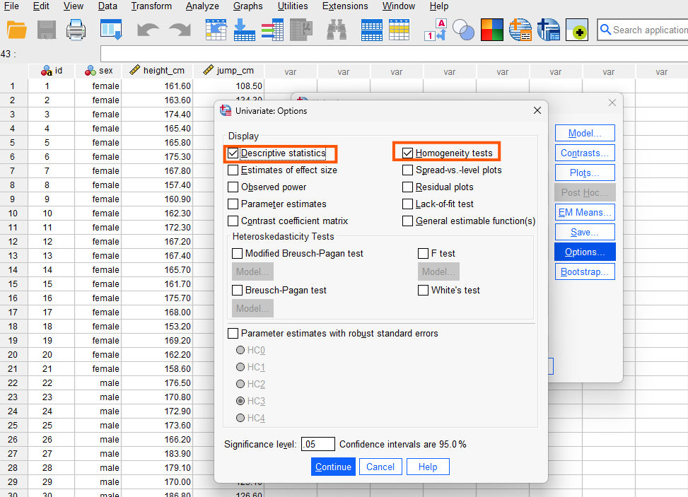
In the Option window, we select Descriptive statistics and Homogeneity tests. The homogeneity test produces Levene’s test of homogeneity of variance to check the assumption of equality of variances. We click on Continue and finally on Run to perform ANCOVA and obtain the results in SPSS output window.
Interpreting ANCOVA in SPSS
In this study, the sports scientist was interested in knowing if female and male athletes perform differently in high jump sport. In addition to collecting data on high jump performance and athletes’ sex, the sports scientist also collected data on athletes’ heights to see if any difference in jump performance could also be explained by athletes’ heights. Therefore, the researcher first performed an ANOVA to compare high jump performance difference between female and male athletes and then conducted an ANCOVA to include athletes’ heights as a covariate (for two groups, we can also use the independent samples t-test, but we use ANOVA to compare it with ANCOVA).
Figure 8 shows the results of an ANOVA with sex as the only independent variable (to perform an ANOVA, please see this module on one-way ANOVA in SPSS).
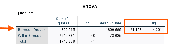
The Between Group row (i.e., between female and male) indicates that there is a significant difference between female and male athletes on high jump performance. Could this result hold if we enter athletes’ heights as a covariate? We can look at the ANCOVA results we just obtained. After the case summary table, we can see the Descriptive Statistics table (Figure 9).
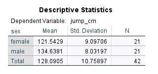
According to these mean values, male athletes on average outperformed female athletes, confirming the results of the ANOVA (without adjusting for any covariates). The next table shows Levene’s equality of error variance assumption test (Figure 10).
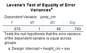
Because the Levene’s test is not statistically significant, we conclude that the error variances between female and male groups are homogenous (similar). ANCOVA is generally robust to mild variance heterogeneity. So, this assumption is met. Next, we can see the main ANOVA results in Tests of Between Subjects Effects table (Figure 11).
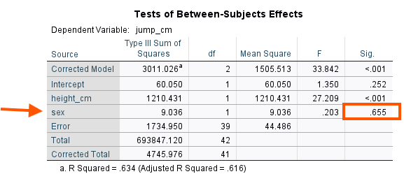
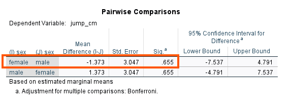
The ANCOVA model takes into account the effect of athletes’ heights and then compares the adjusted means between the female and male groups. According to the ANCOVA results, there is not a statistically significant difference between female and male athletes in high jump performance (p = .655). ANCOVA has recalculated the mean high jump performance for both female and male athletes. The adjusted means are presented in Estimates table (Figure 12).
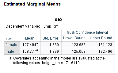
According to the adjusted means, the difference between female and male athletes on high jump performance is negligible. The pairwise comparison results (Figure 13) confirms the non-significant adjusted means difference (p = 0.655).
We can compare the adjusted means with the unadjusted means in the Descriptive Statistics table above, reproduced below in Figure 14.

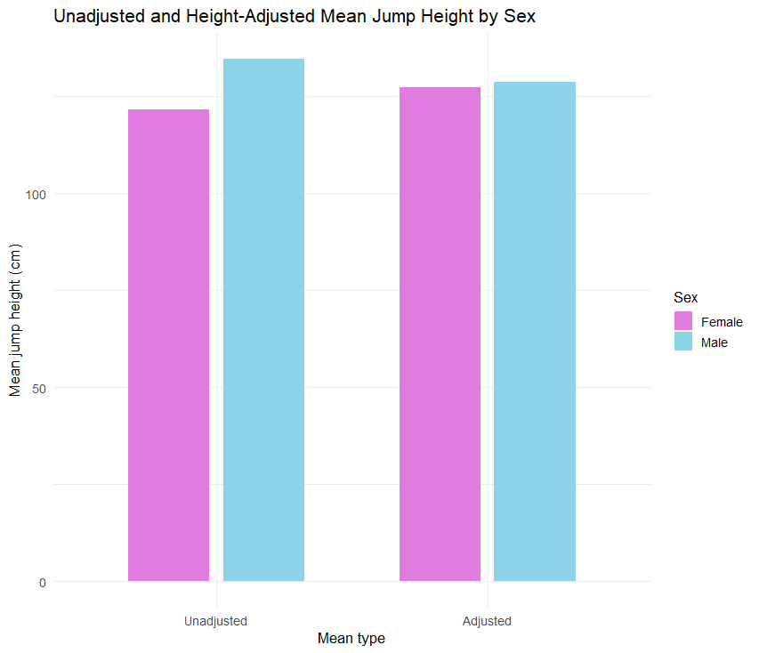
We can see that before adjusting for the heights of the athletes, the mean difference was noticeable, but after adjusting for the heights, the mean difference is negligible and statistically non-significant.
Reporting ANCOVA Results
A sports scientist examined whether male and female high‑jump athletes differ in performance and whether any difference remains after accounting for height. Using data on athletes’ sex, height, and jump height, the researcher first ran a one‑way ANOVA, which showed that males appeared to outperform females. An ANCOVA was then conducted with height as a covariate. After adjusting for height, the sex effect was no longer statistically significant (p = .655), and the adjusted means for males and females were nearly identical, indicating that the initial difference was largely explained by height rather than sex.