SPSS FOCUS
A comprehensive guide to statistical analysis in SPSS
Logistic Regression in SPSS
Logistic regression is a statistical method that models the relationship between a set of independent variables and one binary dependent variable. A binary variable has two possible outcomes, such as head or tail, success or failure, having hypertension or not having hypertension. Logistic regression models the nonlinear relationship between the independent variables and the binary outcome variable. Logistic regression is also used for classification purposes in machine learning.
Introduction to Logistic Regression
When the relationship between a continuous dependent variable and a set of independent variables is linear and if the dependent variable data are distributed following a normal distribution, we can model such a relationship using linear regression. However, in some research studies, our dependent variable is not continuous, such as when our dependent variable represents two discrete values like pass / fail, recovered / not recovered, have diabetes / does not have diabetes, spam / ham.
The implication of a binary variable as a dependent variable is that we cannot use linear regression to model the relationship between a binary variable and other independent variables because the relationship is not linear (it is nonlinear).
In the following sections, we present an example research scenario where a logistic regression will be used to model the relationship between an independent variable and a dichotomous outcome variable. We will demonstrate how to perform a logistic regression in the SPSS program step-by-step and how to interpret the SPSS results from the logistic regression analysis.
Logistic Regression Example
Does blood pressure predict diabetes in female patients?

A public health researcher is interested in understanding what predictor variables are related to diabetes in female patients and if such variables have a strong relationship to indicate a warning predictor for the diabetes condition.
For this purpose, the researcher collects data from a sample of ethnic population on the blood pressure, glucose level, and body mass index (BMI), and whether or not the participants have diabetes (a dichotomous dependent or outcome variable).
Table 1 includes values for blood pressure, glucose level, and body mass index (BMI) and diabetes status (0 = without diabetes; 1 = with diabetes) for five participants. (These data are from the Pima Indians Diabetes Dataset, originally published by the National Institute of Diabetes and Digestive and Kidney Diseases, collected from 768 female participants from Arizona, USA.)
| Patient | Blood Pressure | Glucose Level | BMI | Diebetese Status |
|---|---|---|---|---|
| Patient 1 | 66 | 89 | 28.1 | 0 |
| Patient 2 | 50 | 78 | 31.0 | 1 |
| Patient 3 | 70 | 197 | 30.5 | 1 |
| Patient 4 | 60 | 89 | 30.1 | 1 |
| Patient 5 | 72 | 166 | 25.8 | 1 |
| … | … | … | … | … |
The data for this example can be downloaded in SPSS format or in CSV format. In this example, we select only blood pressure as the independent (predictor) variable. The complete dataset has more variables (with missing values denoted by 0).
Entering Data into SPSS
The data for this example can be downloaded from the links above. If you have downloaded the SPSS format of the data, double-click on the file to open the file and the SPSS program. Alternatively, you can open the file through SPSS menu bar using the File / Open / Data. If the downloaded file is in the CSV format, in SPSS you can use File / Read text data to open a step-by-step window (wizard) to open the CSV file.
To enter the data in the SPSS program manually (entering data by hand or pasting the data into SPSS from a spreadsheet), first we click on the Variable View tab (bottom left) and create the variables under name column: Patient, BloodPressure, and Diabetes. We specify the following attributes for each variable:
- Patient: Type is string. Width is 16. Measure is Nominal.
- BloodPressure: Type is Numeric. Measure is Scale.
- Diabetes: Type is Numeric. Measure is Nominal.
These are our main variables in this example. The data file has more variables, including pregnancies, glucose level, insulin, etc.
When defining the variables, we specify both the data type and the measurement level for SPSS. The data type is used by the SPSS software to understand the data type and structure (e.g., text, numbers, dates, etc.), while the measurement level helps the statistical algorithm for running the appropriate analysis.
In our data, the Patient variable consists of patient names or IDs and is not included in computation; therefore, we select “String” as the data type and “Nominal” (i.e., not a number) as the measurement level. For the BloodPressure variable, we choose Numeric for its data type and Scale for its measurement level. For the outcome variable Diabetes, we choose Numeric as its data type and Nominal as its measurement level.
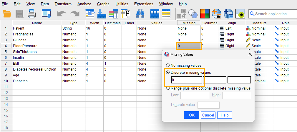
Because our data have missing values shown by the number 0 in some independent variables, we need to tell SPSS that the 0 values in Blood Pressure are missing values and not actual observed blood pressure values (Note: In the original dataset, 0 indicates missing values for several variables; in this tutorial, we only consider Blood Pressure missing values because it is the only predictor used.) Therefore, for the Blood Pressure variable, we click on Missing and in the window that opens select Discrete missing values and enter 0 in the first box, as shown in Figure 1.
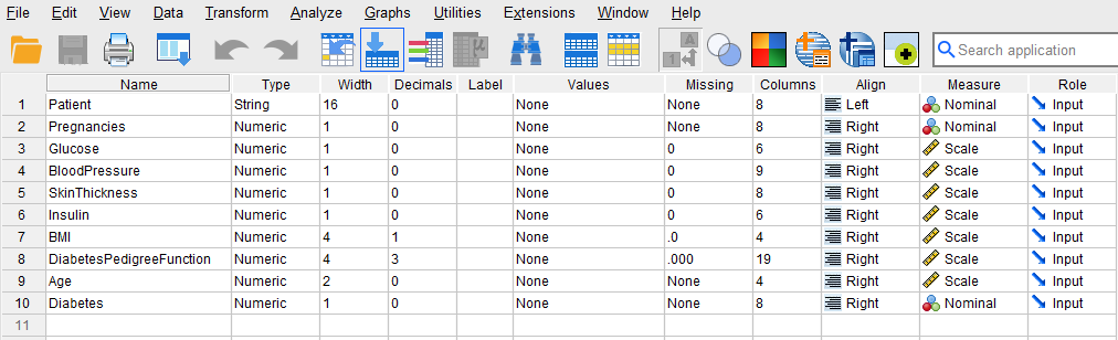
After creating all variables, the Variable View tab of SPSS for our dataset should look like Figure 2.
Once the variables are created, we can enter / paste the data into the columns Patient, BloodPressure, and Diabetes in the Data View tab of SPSS program (the data can be downloaded from the links above, so no need to enter the data manually because it is a bit large).
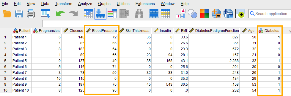
For Patient, we can enter their names or an ID. For the variable BloodPressure, we enter the pressure measurements of the patients. Finally, for the variable Diabetes, we enter 0 if the patient does not have diabetes and 1 if the patient has diabetes. Figure 3 shows how the data for all three variables should look like in the Data View tab.
We are now ready to run a logistic regression analysis in SPSS!
Analysis: Logistic Regression in SPSS
Logistic regression is a statistical technique for modeling the relationship between a set of independent variables and a binary dependent or outcome variable.
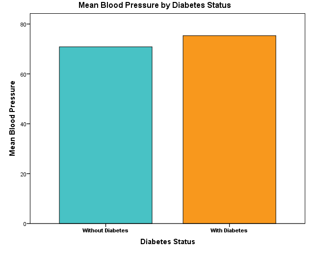
In our example research study, a public health researcher is interested in modeling the relationship between Blood Pressure (the independent variable) and Diabetes (the dependent or outcome variable) in female patients. Figure 4 shows that patients with and without diabetes have different mean blood pressure values.
To model this relationship, the researcher collects data on some health indicators, including blood pressure and whether the patients have diabetes. The researcher uses the logistic regression model because the dependent variable (diabetes) is binary with two possible values of 0 and 1 (where 0 = without diabetes, and 1 = with diabetes).
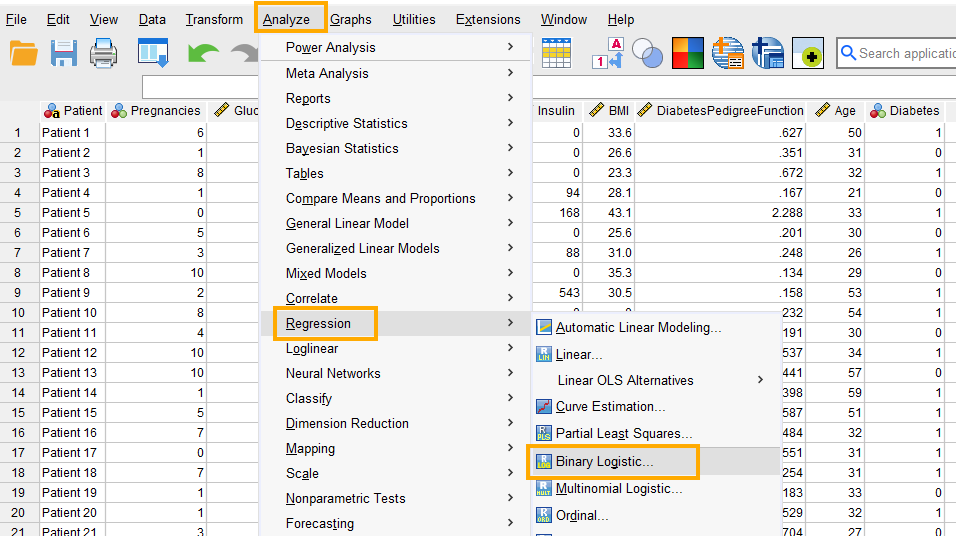
In SPSS, logistic regression can be accessed through the menu Analyze / Regression / Binary Logistic. So, as Figure 5 shows, we click on Analyze and then choose Regression and then Binary Logistic.
After clicking on Binary Logistic, a window will appear asking for Dependent and Covariates (independent variables) we want to model using logistic regression (Figure 6). We send Diabetes into the Dependent box and Blood Pressure into the Covariates box.
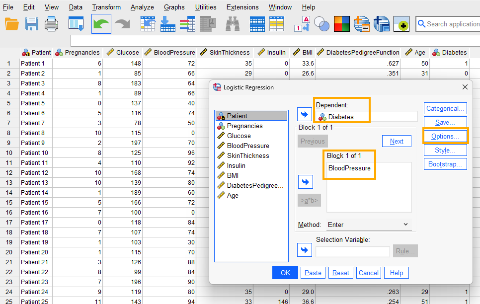
Next, we click on Options to choose the Hosmer-Lemeshow goodness-of-fit test and CI for exp(B) (confidence intervals for the regression coefficient estimates on odds scale) (Figure 7).
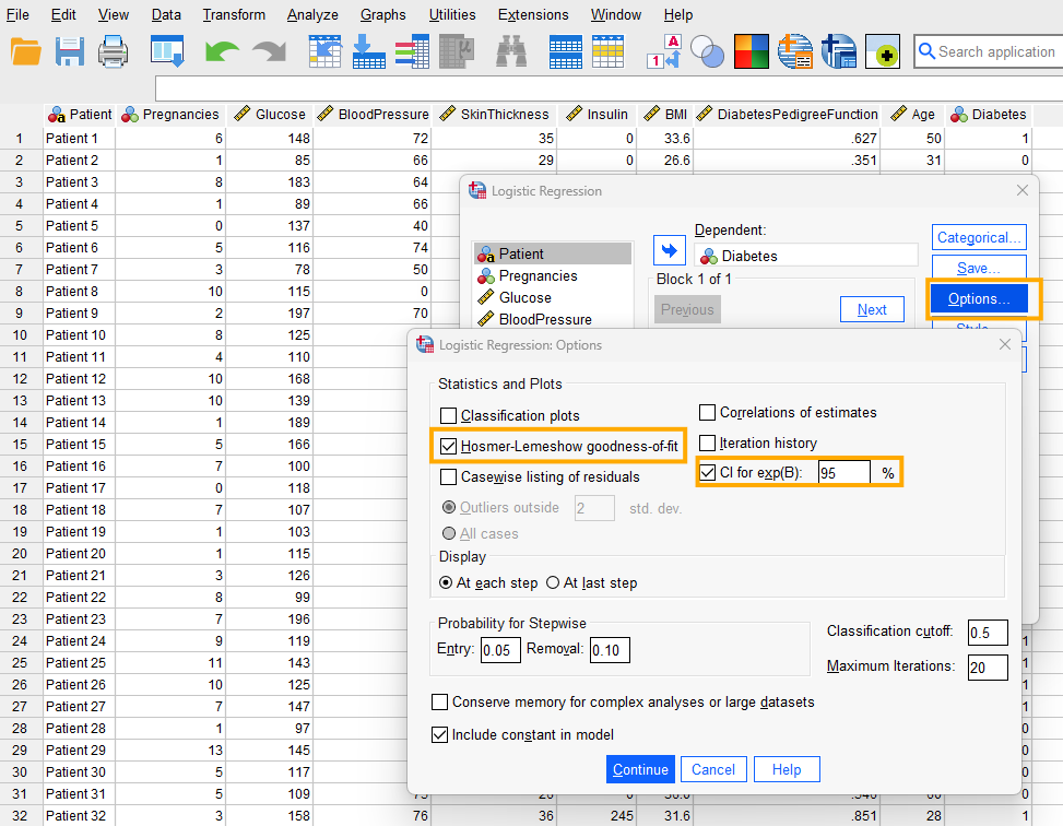
The Hosmer-Lemeshow test in logistic regression with a binary outcome variable assesses how well our model fits the data. A good model has no or very little deviance from the ideal theoretical model, hence a p > 0.05 shows that the model is not significantly different from an ideal model and therefore is a good fit. We click on Continue to close the Options window and lastly click on OK to run the logistic regression test in SPSS. The results of the logistic regression analysis are printed out in the Output window.
Interpreting Logistic Regression in SPSS
The first table in the output (Figure 8) is the Case Processing Summary.
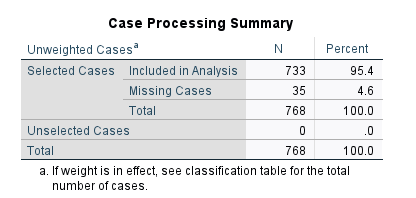
Case Processing Summary includes the total number of cases in the data set (n = 768), the number of missing values (n = 35), and the number of valid values used in analysis (n = 733) and their corresponding percentages.
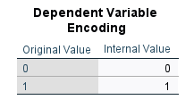
The next table (Dependent Variable Encoding, Figure 9) shows the values of the dependent variable, which are 0 (without diabetes) and 1 (with diabetes).
The rest of the tables in the output are related to the logistic regression analysis results. SPSS divides these tables into two major sections: Block 0 and Block 1. Block 0 includes all tables in the logistic regression results when there is no independent variable in the model. The only estimate in the model is the constant. Therefore, the results in Block 0 tables do not help us understand the effect of the independent variable (Blood Pressure). Figure 10 shows the tables in Block 0.
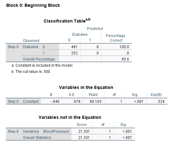
In Block 0, the Classification Table shows the actual number of patients without diabetes (0) and with diabetes (1) and the model prediction using only the constant. The next table is Variables in the Equation, which includes only the constant or the intercept. In our example, the intercept is -0.646, meaning that the log odds of having diabetes (compared to not having diabetes) is -0.646.
This provides a baseline log odds, based only on the proportions of 1 and 0 values in the data. The antilog (exponentiation) of -0.646 is 0.524 (the last column in Variables in the Equation table, Exp(B)), which means the odds of having diabetes by just looking at the proportions of 1 and 0 in the data is 0.524 versus not having diabetes. We can convert odds to probability: Prob (having diabetes) = 0.524 / (1 + 0.524) = 0.34. So, the probability of having diabetes is 0.34 based only on the proportions of patients with and without diabetes, and without considering any predictors, such as blood pressure, age, sex, etc. But we are interested in the effect of a predictor, so we rarely use a constant for prediction.
The last table shows Variables not in the Equation, which is our predictor the Blood Pressure. To understand the effect of the Blood Pressure, we need to look at the tables in the Block 1 of the output.
The first table in Block 1 is the Omnibus Tests of Model Coefficients (Figure 11).
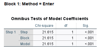
This table shows that our overall (omnibus) model (including all variables) is statistically significant with a chi-square value of 21.615, degrees of freedom of 1, and p < 0.01 (Sig.=.000).
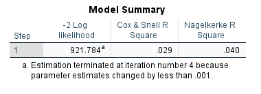
The next table, Model Summary, in Figure 12 shows the amount of variance in the outcome (Diabetes) that is explained by the predictor (Blood Pressure). The Cox and Snell R Square and Nagelkerke R Square are both measures of explanatory power of the predictor variable. According to the Nagelkerke R Square, the predictor Blood Pressure can only explain about 4% of the variance in the outcome variable. The -2 Log Likelihood statistic shows how fit the model is. This statistic is used relative to another model (such as the null model). The model with lower -2 Log Likelihood is then chosen as the better model in terms of fit.
The Hosmer-Lemeshow goodness-of-fit statistic that we requested in the options is shown in the following table in Figure 13.
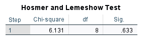
The Hosmer-Lemeshow goodness-of-fit statistic is based on the chi-square distribution. With a chi-square value of 6.131 (df = 8), the Hosmer-Lemeshow goodness-of-fit value is not statistically significant (p = 0.633), indicating that the model has good fit and is not significantly different from an ideal model.
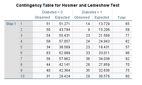
Hosmer-Lemeshow goodness-of-fit statistic divided the data into several batches (bins) and compares the observed frequency with expected frequency (predicted probability) in each level of the outcome variable. Figure 14 shows that Hosmer-Lemeshow goodness-of-fit test had divided the data into 10 bins.
The next table, Classification Table (also known as the confusion table, especially in machine learning context), shown in Figure 15, includes the model performance in correctly predicting an outcome.
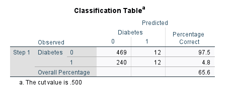
A good model should show a high number in (0, 0) and (1, 1) cells (the numbers on the diagonal). A (0, 0) value shows the number of correct predictions of not having diabetes (True Negative). In this table, the model was correct 469 times but was incorrect (confused) in 12 predictions (predicted 0 as 1, upper right cell). The model is only correct in predicting a 1 as a 1 (True Positive) 12 times and was incorrect 240 times (predicted diabetes as not diabetes). The accuracy of the model is 65.6%, which shows the proportion of correct predictions.
The values in the Classification Table are usually expressed as accuracy, precision, sensitivity, and specificity metrics.
- Accuracy: proportion of total correct predictions (65.6%)
- Sensitivity (or recall): ability to correctly identify positive cases of diabetes (4.8%, which is too low, but common in models with only one weak predictor)
- Specificity: ability to correctly identify negative cases of diabetes (97.5%)
- Precision: proportion of positive cases that were predicted to be positive or positive predictive value (50%).
In imbalanced datasets (like the Pima data in our example), though, accuracy can be misleading; sensitivity and specificity should be interpreted together.
The last table in Block 1 is the Variables in Equation table (Figure 16), which includes the regression coefficients for the model.
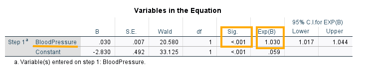
The predictor in our model is Blood Pressure, with a coefficient B = 0.030, which is statistically significant (Wald test value = 20.580, df = 1, Sig. = .000).
In logistic regression, we usually interpret the results in comparing one value of the outcome against the other value. For example, we want to know what are the odds of having diabetes against not having diabetes. We are usually interested in the odds and probability values.
The B value of 0.30 in the table is in the log odds (logit) scale. So, we take the antilog function to transform from log odds scale to odds scale. To do so, we exponentiate the log odds. Exponentiation results in antilog. The last two columns in the table show that Exp(B) = 1.030 (on odds scale) with 95% confidence intervals values between 1.017 and 1.044. Because the confidence interval does not include the value of 1 (equal odds), we can conclude that the predictor has a statistically significant effect. Generally, if the odds value is larger than 1, it shows an increase, while if the odds value is less than 1, it shows a decrease. Odd value of 1 indicates no effect.
The coefficient for Blood Pressure on log odds scale is interpreted as follows: for one unit increase in blood pressure, the log odds of having Diabetes increases by 0.03. The Blood Pressure coefficient on the odds scale is 1.030 and is interpreted as: for one unit increase in blood pressure, the odds of having diabetes multiplies by 1.030.
We can convert odds to percentage increase by subtracting 1 from odds (in this case, 1.03 -1 = 0.03) and multiplying by 100. So, the odds of having diabetes increases by around 3% when blood pressure increases 1 unit.
The constant (or intercept) value on log odds scale is -2.830 and on odds scale is 0.059. The constant is usually not interpreted alone. In general, the constant is interpreted as: when Blood pressure is zero, the log odds of having Diabetes is -2.830 and the odds are 0.059. But blood pressure (or any other physical predictors, such as height or weight) may never be zero. So, we usually do not interpret the constant alone (in fact, SPSS allows you to eliminate the constant from the results in the Options menu).
Similar to linear regression, we can write the result of the logistic regression analysis as an equation (model):
Predicted Log Odds of Diabetes = -2.830 + 0.030*(Blood Pressure)
Remember that the equation above returns an expected value in log odds (or logit). To obtain the odds, we need to exponentiate the result, as demonstrated in the following example.
Suppose a female patient’s blood pressure is 90. We predict the log odds of her having diabetes to be:
Predicted Log Odds of Diabetes = -2.830 + 0.030*(90) = -0.130
So, the log odds of having diabetes for a female patient with blood pressure of 90 is estimated to be -0.130. We exponentiate the log odds to remove log and get the odds only. The exp(-0.130) = 0.878, which is less than 1, which means a decrease. So, the odds of developing diabetes for a female patient with blood pressure of 90 is 0.878.
In addition to odds, we can also calculate the probability of having diabetes with a blood pressure of 90. To calculate our prediction in terms of probability, we use the following equation:
Probability = Odds / (1 + Odds)
In our example, we calculated odds of developing diabetes with a blood pressure of 90 to be 0.878, so the probability of having diabetes for a female patient with blood pressure of 90 is,
Probability of Having Diabetes = Odds / (1 + Odds) = 0.878 / (1 + 0.878) = 0.468
The probability of having diabetes for a patient with a blood pressure of 90 is about 0.47.
Reporting Logistic Regression Results
A logistic regression analysis was conducted to examine the relationship between blood pressure and diabetes status (0 = no diabetes, 1 = diabetes) in a sample of 768 female patients. The results indicated that blood pressure was a significant predictor of diabetes status (B = 0.03, p < 0.05). The odds ratio for blood pressure was 1.030, indicating that for each 1-unit increase in blood pressure, the odds of having diabetes increased by 3%. The model had a good fit, as indicated by the Hosmer-Lemeshow test (p > 0.05).