SPSS FOCUS
A comprehensive guide to statistical analysis in SPSS
Simple Regression in SPSS
Simple regression is a statistical method that measures and models the relationship between one independent variable and a continuous dependent variable. The independent variable (or predictor) can be continuous or discrete (categorical). Modelling means obtaining an equation from data that can be used to predict a future outcome. Regression is a fundamental method in predictive modeling.
Introduction to Simple Regression
The relationship between two random variables can be established using several measures of association and relationship, including Pearson correlation, Spearman correlation, or Kendall Tau correlation. These correlation methods provide us with the strength and direction of a relationship summarized as a single number (correlation coefficient). These measures of association help us establish the existence and strength of a relationship. However, they stop there and cannot help us to predict a future value because they do not provide us with a prediction formula (a model).
In a linear relationship, regression analysis uses the (intercept-slope) equation of a line to establish the relationship between two variables. Therefore, like a line equation, a linear regression equation has an intercept (where the line crosses the vertical or y-axis) and a slope (how fast the values of the y-variable change as a function of the values of the x-variable). The slope of the line shows the relationship between the independent and the dependent variables: if the slope is large, the relationship is strong (and the other way round), and if the slope is negative, the relationship is inverse. The slope of the line is called the coefficient and is denoted by the letter b. The intercept is also shown by the letter beta (β). In a simple linear regression analysis, we are mostly interested in the coefficient (slope).
In a linear regression analysis, the variable whose values we model and try to predict is called the dependent variable (usually shown by the letter “y”), and the variable that is used to predict those values is called the independent variable (usually shown by the letter “x”). Other names for the dependent variables are the response, the outcome, or the target variable. Other names for the independent variable are the predictor, the explanatory variable, or the feature. Unlike correlation analyses, in a regression model we need to designate which variable is the dependent variable (y) and which variable is the independent variable (x).
A regression model is called a simple regression model if there is only one independent variable. If there are two or more than two independent variables, the regression is called a multiple regression model. The dependent variable in a simple or multiple regression is continuous (on the interval or ratio scale of measurement). However, the independent variables can be continuous, binary (two levels, like gender: male and female), or categorical (more than two levels, such as income: low income, middle income, and high income).
In the following sections, we present an example research scenario where a simple linear regression will be used to analyze the data. We will demonstrate how to perform a simple linear regression in the SPSS program step-by-step and how to interpret the SPSS results from a simple linear regression analysis.
Simple Regression Example
What is the relationship between the number of hours students dedicate to studying and their test scores? Can the number of study hours predict test scores?

A high school teacher is interested in modeling the relationship between the number of hours students dedicate to studying and the scores the students achieve on their tests. The teacher randomly selects 65 students from the school district and asks the students how much time per week they spend preparing for their test. The teacher is not only interested in understanding the relationship between study hours and test scores, but also if the number of studies can be used to predict a student’s test score. Table 1 includes the scores of five students on the test.
| Student | Study Hours | Test Score |
|---|---|---|
| Student 1 | 31 | 70 |
| Student 2 | 32 | 75 |
| Student 3 | 44 | 100 |
| Student 4 | 32 | 80 |
| Student 5 | 28 | 83 |
| … | … | … |
The teacher enters the data in the SPSS program in the computer lab. The data for this example can be downloaded in the SPSS format or in CSV format.
Entering Data into SPSS
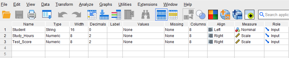
To enter the data in the SPSS program, first we click on the Variable View tab (bottom left) and create three variables under name column: Student, Study hours, and Test score. We specify the following attributes for each variable:
- Student: Type is string. Width is 16. Measure is Nominal.
- Study_Hours: Type is Numeric. Measure is Scale.
- Test_Score: Type is Numeric. Measure is Scale.
When defining the variables, we specify both the data type and the measurement level for SPSS. The data type is used by SPSS software to understand the data type (e.g., text, numbers, dates, etc.), while the measurement level helps the statistical algorithm for running the appropriate analysis.
In our data, the Student variable consists of student names or IDs and is not included in computation; therefore, we select “String” as the data type and “Nominal” (i.e., not a number) as the measurement level. We increase the Width of the Student variable to 16 characters so that the full names for longer names are shown. For the two continuous variables Study_Hours and Test_Score, we choose Numeric for their data types and Scale for their measurement levels. SPSS uses the term scale for both interval and ratio measurement levels. After creating all variables, the Variable View panel of SPSS for our dataset should look like Figure 1.
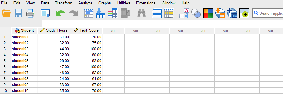
Once the variables are created, we can enter the data into the columns Student, Study_Hours, and Test_Score in the Data View tab of SPSS program. For Student, we can enter their names or an ID. For the variable Study_Hours, we enter the number of hours each student reports studying. Finally, we enter the test scores in Test_Score column for each student. Figure 2 shows how the data for all three variables should look like in the Data View tab.
Now we are ready to conduct a simple regression analysis in SPSS!
Analysis: Simple Regression in SPSS
Simple linear regression is a predictive modeling technique for modeling the relationship between one independent variable and a dependent variable for the purpose of predicting future values and understanding the direction, strength, and significance of the relationship between an independent variable and a dependent variable.
In our example research study, a teacher is interested in modeling the relationship between the number of weekly hours students spend studying (the independent variable) and their test scores (the dependent variable). To investigate this relationship, the teacher collects data on the study hours and test scores from a random sample of 65 students. The teacher uses the simple linear regression method because there is only one independent variable and one dependent variable.
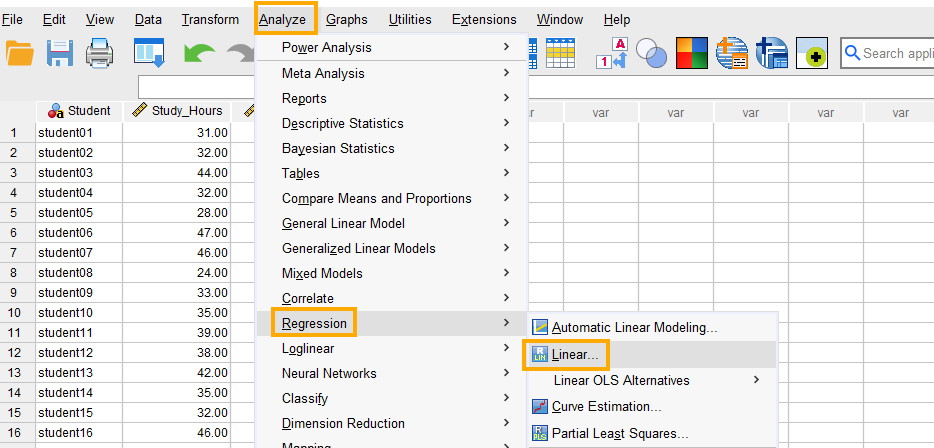
In SPSS, the simple linear regression can be accessed through the menu Analyze / Regression / Linear. So, as Figure 3 shows, we click on Analyze and then choose Regression and then Linear.
After clicking on Linear, a window will appear asking for Dependent and Independent(s) variables we want to model using simple regression (Figure 4). We send Test_Score into the Dependent box and Study_Hours into the Independent(s) box.
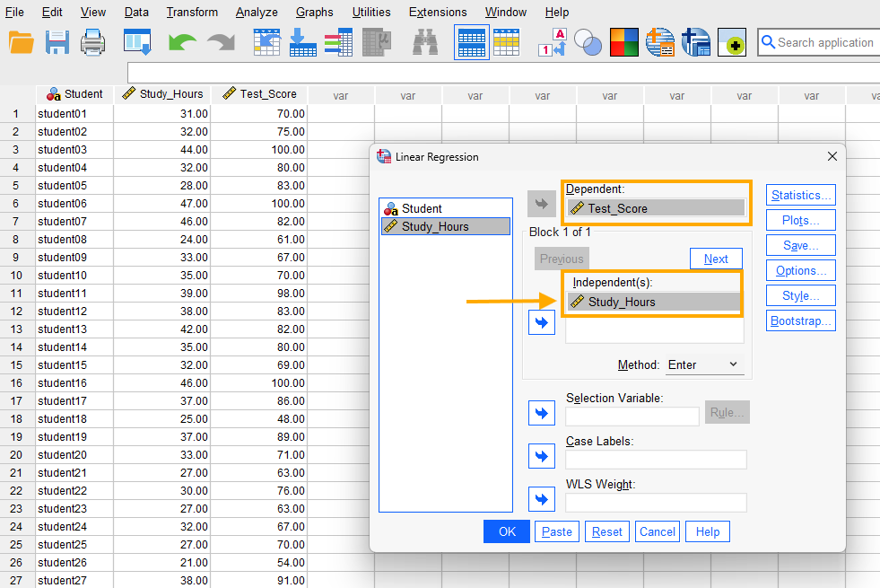
Finally, we click on OK to run the simple linear regression analysis. SPSS will produce the results of the simple linear regression analysis in the Output window.
Interpreting Simple Regression in SPSS
In our example research study, a teacher is interested in investigating the relationship between the number of weekly hours students spend studying and their test scores. In this example, the dependent variable is the students’ test scores and the independent (predictor) variable is the number of study hours. The teacher runs a simple linear regression in SPSS and obtains several tables in the Output file.
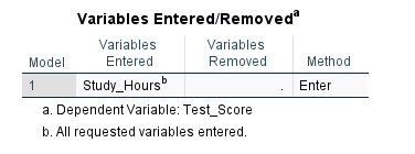
The first table in the output (Figure 5) shows the names of the independent and dependent variables analyzed by simple regression.
Next, the Model Summary table (Figure 6) shows the relationship between Study hours and Test scores using R, R Square, and Adjusted R Square statistics.
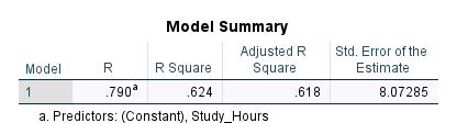
In linear simple regression, the R statistic is equivalent to the Pearson correlation coefficient which in this example measures the relationship between Study hours and Test scores. As we stated in the introduction, besides predictive modeling, a regression analysis can also show the relationship (and direction and significance of the relationship) between variables. In our example, the correlation between Study hours and Test scores is 0.79, which is relatively high and positive.
The R Square statistic (also known as the coefficient of determination) shows the amount of variance in the dependent variable explained by the independent variable(s). In other words, the R Square statistic shows how much information the independent variable brings to our model (and how much is left out). The higher the R Square, the more informative the independent variable is. The R Square values can also be used to compare different regression models to understand which model better explains the variability in the outcome variable. Adjusted R Square takes into account factors that inflate R Square, such as the number of independent variables. So, we recommend looking at Adjusted R Square as a more unbiased measure of the informativeness of our independent variables. In this example, R Square is 0.62, implying that Study hours alone can explain 62% of the variance in the dependent variable in the model and about 38% of variance (1 – 0.62 = 0.38) remains unaccounted for or unexplained.
Next, the ANOVA table (Figure 7) looks at regression from an analysis of variance perspective where different forms of variances (sum of squares) are reported.
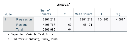
The ANOVA table provides two sources of variance and calls them Sum of Squares: Regression sum of squares and Residual sum of squares. The Regression part shows the information, and the Residual part shows noise or unknown information. We want a high information to noise ratio (also known as signal to noise ratio, SNR). The higher this ratio, the more likely our model will be statistically significant and meaningful. In this ANOVA table, we can see that F = 104.360 and is statistically significant. So, our regression model (i.e., choice of independent variables, data) is statistically good.
The statistics needed to model the relationship between Study hours and Test scores are present in the Coefficients table (Figure 8).
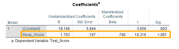
There are two rows in the table: Constant and Study hours, each with a B value (18.166 and 1.702, respectively). The B values are the coefficients of the regression model and come in two versions: unstandardized and standardized. The unstandardized version is on the original scale of the independent variable measurement while the standardized version has been scaled to vary between -1 and 1.
In this table, Constant is the intercept, which is the point on the Y axis (the dependent variable) where the regression line passes through (where X or the independent variable equals 0). In our example, the intercept is 18.166, meaning that when study hour is zero, we theoretically expect the test score to be 18.166 on average.
The next row in the Coefficients table shows the coefficient for the independent variable Study hours. The coefficient B (1.702) is the measure of relationship between the independent variable and the dependent variable. In our example, the coefficient for the independent variable 1.702, which is positive, and which is statistically significant. This means there is a positive and statistically significant relationship between Study hours and Test scores. The coefficient for the independent variable Study hours is interpreted as follows: for each one hour of study, the test score increases on average 1.702 scores. We say increases because the coefficient is positive. The standardized version of the coefficient in a simple linear regression can be interpreted as a Pearson correlation coefficient. So, in our example, the correlation between Study hours and Test scores is 0.79.
Now that we have regression model coefficients, we can build our model. We can write the result of the analysis in terms of the relationship between the test score and study hours as the following equation (model):
Predicted Test Score = 18.166 + 1.702 * Study_Hours
In this equation, the value 18.166 is the Constant (intercept) from the coefficients table above and the value 1.702 is the coefficient for the independent variable Study hours. To predict a new test score, we replace Study hours with a number (for example 25 hours) and calculate the expected test score. For example, if an individual studies for 25 hours a week (Study hours = 25), we predict their expected test score to be:
Predicted Test Score = 18.166 + 1.702 * 25 = 60.72
This means that if a student studies for 25 hours, we expect their test score to be approximately 60.72.
As another example, if a student studies for 35 hours (Study hours = 35), we predict their expected test score to be:
Predicted Test Score = 18.166 + 1.702 * 35 = 77.74
This means that if a student studies for 35 hours, we expect their test score to be approximately 77.74.
The simple linear regression equation is based on the intercept-slope equation of line. So, after fitting the model, we can plot our data in a scatter plot and draw the regression line (also called the line of best fit) and observe how near or far our actual data are from theoretical predictions (Figure 9).
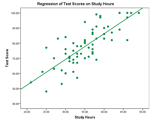
The scatter plot in Figure 9 shows that there is a positive relationship between Study hours and Test score. The line in the plot is the regression line (or the line of best fit). The closer the actual data points are to the fit line, the better the model is (the less difference between actual data and predicted values).
Reporting Simple Regression Results
In this research, we aimed to explore the relationship between the number of hours students dedicate to studying and their test scores. To investigate this, we selected a random sample of 65 students and collected data on the hours they spent studying and their corresponding test scores.
The results of the simple regression analysis revealed that study hours significantly influence test scores (b = 1.702, p < 0.05). The coefficient of determination, R²=0.62, highlights that approximately 62% of the variation in test scores is explained by study hours. This suggests a moderately strong relationship, emphasizing the impact of dedicated study time on academic performance.
These findings underline the importance of consistent study habits in achieving higher test scores. The positive slope of the regression equation suggests that every additional hour spent studying results in an average increase of 1.702 points in test scores. These insights offer valuable guidance for both students and educators, demonstrating the significance of strategic time management in enhancing academic outcomes.