SPSS FOCUS
A comprehensive guide to statistical analysis in SPSS
Chi-squared Test in SPSS
The chi-squared test of independence is a statistical test that measures the relationship between categorical variables. For example, when we are interested in the relationship between two binary or categorical variables, we can use the chi-squared test of independence or association. The chi-squared test of independence is also known as the Pearson’s chi-squared test of independence or association.
Introduction to Chi-squared Test
A Pearson’s chi-squared test of independence or association measures the relationship or the association between categorical variables, such as the association between smoking (smoker, nonsmoker) and heart problems (with heart problems, without heart problems), or the relationship between sex (male, female) and house ownership (own, not owning). Each categorical variable could have two or more than two categories. The categories could be ordered or unordered (nominal).
In a chi-squared test of independence or association, the term association means a relationship but mostly used for describing the relationship between categorical variables. By independence, we mean we want to test if two categorical variables do not depend on each other (i.e., they have no relationship, and hence no dependence on each other).
The data for the chi-squared test may come into two formats: raw count data and a summary count table. For example, suppose we are interested in knowing if there is an association between sleep position (with two values: sleeping on side, sleeping on back) and having backache (with two values: no backache, with backache). We randomly ask 55 patients if they have backache and what their sleep positions are. Each patient provides an answer to the backache question (with / without backache) and sleeping position question (sleeping on side, sleeping on back). We can populate these values in a table like Table 1 below.
| Patient | Sleep position | Back pain |
|---|---|---|
| Patient 1 | Side | No |
| Patient 2 | Side | Yes |
| Patient 3 | Back | No |
| Patient 4 | Back | Yes |
| Patient 5 | Side | Yes |
| … | … | … |
Another way to present data for the chi-squared test of independence or association is to use summary, contingency, or crosstab tables. Each contingency table has as many rows and columns as the number of levels or categories in each variable. For example, in the sleep position and backache data, we have two categories for sleep position (sleeping on side or on back) and two categories for backache (with or without backache). So, we have a 2 x 2 contingency or crosstab table. Each cell of the table includes the total number of co-occurrences of the levels of the variables. The word “contingency” here means dependence because the values of one variable could depend on the values of the other variable (a chi-squared test will show if there is such a dependency and if such a dependency is statistically significant). Table 2 illustrates a contingency table for the sleep position and backache data.
| Sleep Position | Back Pain No | Back pain Yes |
|---|---|---|
| Back Sleepers | 18 | 8 |
| Side Sleepers | 7 | 22 |
Contingency tables, like Table 2 above, are usually read by row. For example, in Table 2, the row “Back sleepers” tells us that among those who sleep on their backs, 18 patients experienced no backache, and 8 patients did experience backache. In row “Side sleepers”, 7 patients didn’t experience backache, but 22 patients experienced backache. Apparently, Side sleepers had more backache complaints (22) compared to Back sleepers (8). So, is there a relationship between sleep position and backache complaints?
In the following sections, we present an example research scenario where the chi-squared test of independence or association will be used to analyze the data. We will demonstrate how to perform the chi-squared test of independence in SPSS step-by-step and how to interpret the SPSS results for the chi-squared test of independence or association.
Chi-squared Test of Independence Example
Is there a relationship between Sleep position (sleeping on side versus on back) and Backache complaints?

A public health researcher is interested in knowing if sleep position is associated with backache. The researcher randomly recruits 55 patients and asks them if they complain about backache and what sleep position they primarily had during the last year. Table 3 includes the responses to the two questions (Sleep position? 0 = Back, 1 = Side; Backache? 0 = No backache, 1 = With Backache) for five participants in the study.
| Patient | Sleep position | Back pain |
|---|---|---|
| Patient 1 | Side | No |
| Patient 2 | Side | Yes |
| Patient 3 | Back | No |
| Patient 4 | Back | Yes |
| Patient 5 | Side | Yes |
| … | … | … |
The health researcher enters the data in the SPSS program in the computer lab. The data for this example can be downloaded in the SPSS format or in CSV format.
Entering Data into SPSS
To enter the data into the SPSS program, first we click on the Variable View tab (bottom left) and create three variables under name column: Patient, Sleep position, and Backache. We specify the following attributes for each variable:
- Patient: Type is string. Width is 16. Measure is Nominal.
- Sleep_Position: Type is Numeric. Measure is Nominal.
- Back_Ache: Type is Numeric. Measure is Nominal.
When defining the variables, we must specify both the data type and the measurement level for SPSS. The data type is used by the computer to read the data, while the measurement level is used by the statistical program for computation. In this example, the Patient variable consists of names or ID’s, and is not involved in the computation, so we select “string” as the data type and “nominal” as the measurement level.
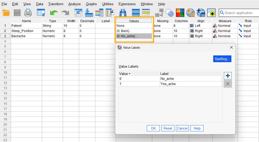
For the variable Sleep_Position, although we use words (Back, Side), we assign numbers to them (e.g., Back = 0, Side = 1). Therefore, we choose “Numeric” as the data type and select “Nominal” as the measurement level. To associate numbers with the sleeping position, in the Value column, click on the cell in the Sleep_position row to open a window. In the Value box, enter 0 and in the Label box, enter “Back,” then click “add.” Repeat this process with Value 1 for the “Side”. Repeat the steps for the variable Backache (0 for No_ache and 1 for Yes_ache). Figure 1 shows how to create these value-label pairs for Sleep position and Backache.
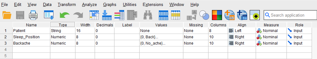
After creating all the variables, the Variable View panel of SPSS for our dataset should look like Figure 2 below.
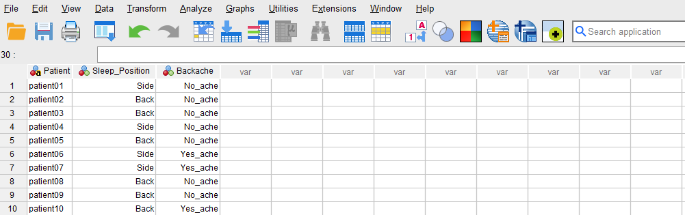
Once the variables are created, we switch to Data View of the SPSS program to enter the data into the columns Patient, Sleep_Position, and Backache. As specified in the Variable View, for Patient we can enter either their names or their ID’s. For the variables Sleep_Position and Backache, we can either directly type the numerical values (0, 1) or their associated labels (e.g., Side, Back; No_ache, Yes_ache). Figure 3 shows how the data for the three variables should look like in the Data View tab.
Now we are ready to run the chi-squared test in SPSS!
Analysis: Chi-squared Test in SPSS
The chi-squared test of independence or association is a statistical method that measures the relationship between categorical variables (counts). In this example, a health researcher investigates the possible relationship between the Sleep position and developing Backache. To explore this, the researcher collects data from a random sample of 55. Each patient indicates their sleep position in the past year and if they had backache.
Because our variables in this example are categorical, the health researcher uses the chi-square test to determine any relationship between Sleep position and Backache.
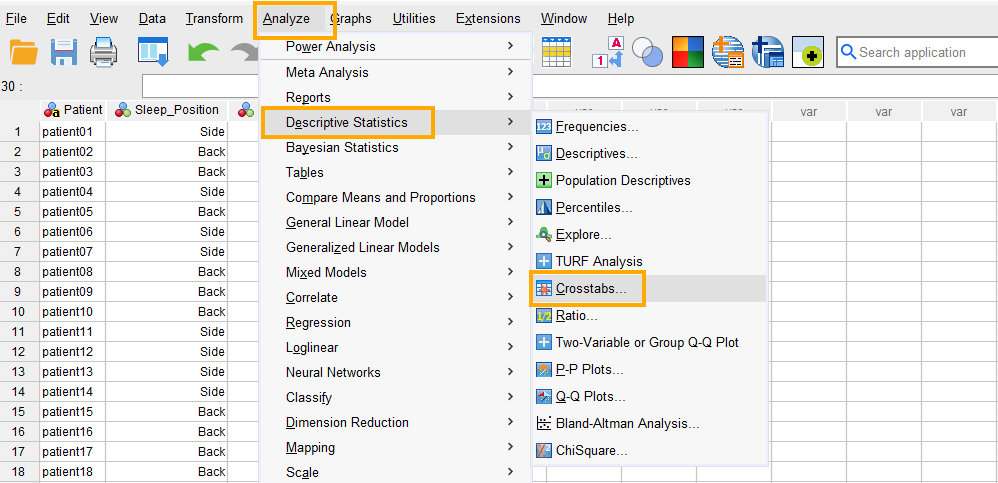
In SPSS, the chi-square test can be accessed through the menu Analyze / Descriptive Statistics / Crosstabs. So, as Figure 4 shows, we click on Analyze and then choose Descriptive Statistics and then Crosstabs item.
After clicking on Crosstabs, a window will appear asking for Row(s) and Columns we want to find an association for (Figure 5). We send Sleep_Position to the Row(s) and Backache to the Column(s) boxes. Although the choice of which variables to send to the row or column will not affect the analysis results, it is good practice to send the assumed independent variable to the rows and the assumed dependent variable to the columns.
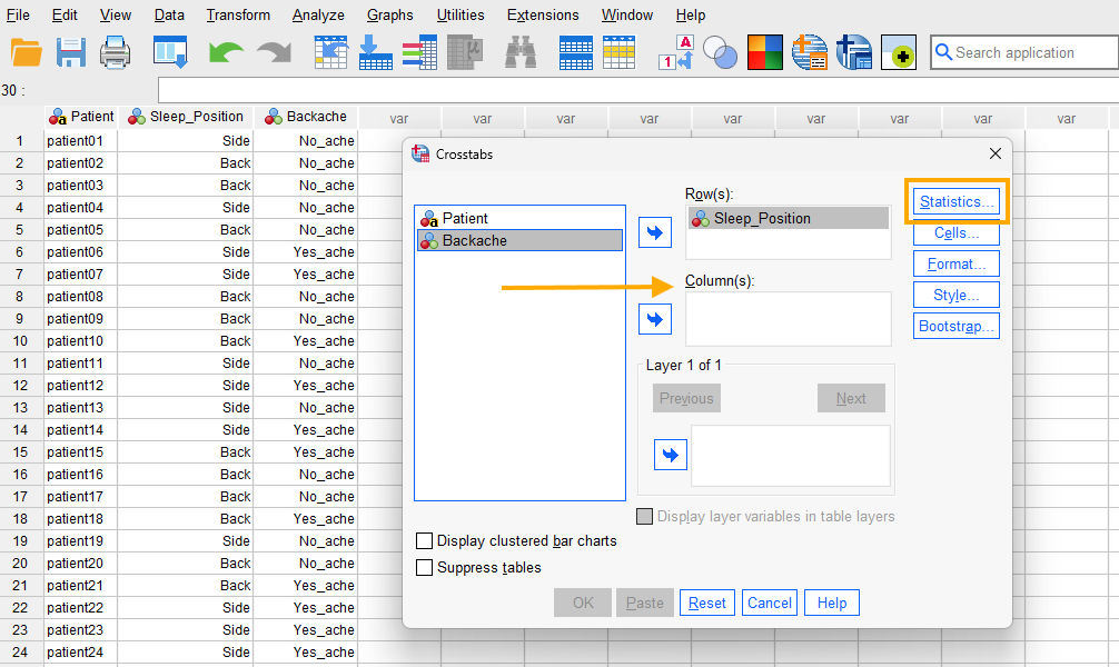
Next, in this window we click on Statistics and in the new window select Chi-square (Figure 6).
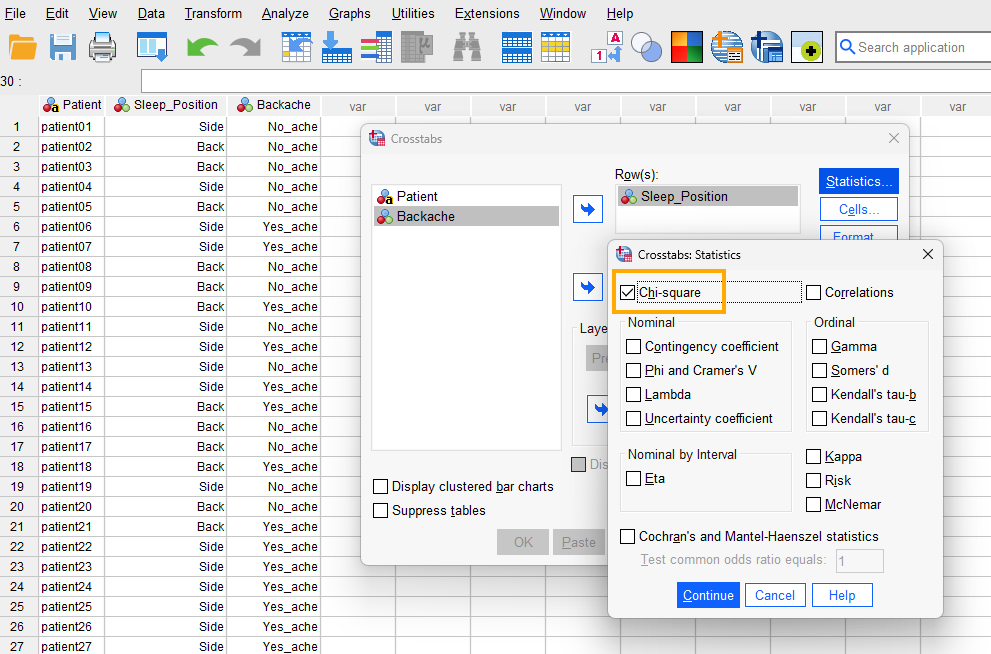
We press Continue and finally click on OK to run the chi squared test. SPSS will produce the results in the Output window.
Interpreting Chi-squared Test in SPSS
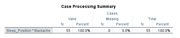
In our example, a health researcher investigates the possible association between Sleep position and having Backache. The researcher runs a chi-squared test of independence in SPSS and obtains several tables in the Output file. The first table (Figure 7 below) simply shows the number of cases (patients) in the data set (valid, missing, and total).
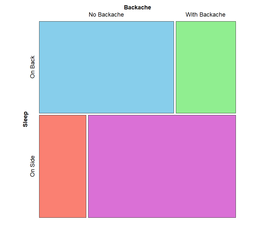
The second table (Figure 8 below) shows the crosstab or the contingency table.
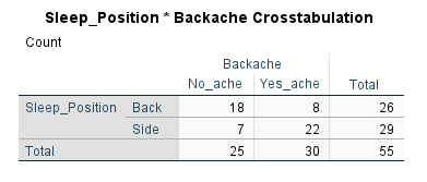
We observe that Sleep position is in the row (independent variable) and Backache is in the column (dependent variable). We usually read a contingency table by rows. In this example, out of 26 patients who slept on their back, 18 did not have backache but 8 had. Out of 29 patients who slept on their sides, 7 did not have backache but 22 did have backache. Because we are interested in backache outcome, we can look at the Backache column and see that out of 30 patients who had backache (in the Yes_ache column), 8 slept on their backs but 22 slept on their sides. This shows an apparent relationship. But we need to look at the Chi-Square Tests table in Figure 9 below to see if the test statistic is significant.
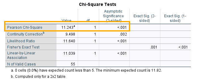
The Chi-square Tests table provides several statistics that measure the independence of Backache variable from Sleeping position. Our main test statistic is the Pearson’s Chi-Square statistic, which is 11.243 and with 1 degree of freedom is statistically significant (p < 0.01).
However, when our contingency table has two categorical variables, each with two levels (a 2 x 2 table), it is recommended to use the Continuity Correction row. This statistic is known as Yate’s correction for continuity. The reason for correction of the Pearson’s Chi-Square is that the chi squared distribution is continuous while the variables are categorical. Therefore, to compensate for some discrepancy, a correction is applied to the Pearson’s chi-squared statistics. We can see that Yate’s correction for continuity gives a chi-square value of 9.498 (p <0 .01), showing a statistically significant association between Sleep position and Backache (the independence hypothesis is not supported).
Reporting Chi-squared Test Results
In this study, we aimed to investigate the relationship between Sleep position and Backache. A random sample of 55 participants was selected. The participants self-reported their sleep position in the past year and whether they had back pain. A chi-squared test of independence was conducted to evaluate the association between sleep position and back pain. The chi-square value of 9.498 (with Yate’s correction for continuity) and a degree of freedom of 1 was statistically significant (p <0 .01). These findings highlight the potential impact of sleep position on back pain.